Panorama Stitching

This article is written by Chahat Deep Singh. (chahat[at]terpmail.umd.edu)

Please contact Chahat if there are any errors.

Table of Contents:

• Introduction
• Adaptive Non-Maximal Suppression
• Feature Descriptor
• Feature Matching
• RANSAC to estimate Robust Homography
• Cylinderical Projection
• Blending Images

Introduction

Now that we have learned about a few building blocks of computer vision from Learning the basics, let us try to do something cool with it! The purpose of this project is to stitch two or more images in order to create one seamless panorama image. Each image should have few repeated local features ($\sim 30-50\%$ or more, emperically chosen). In this project, you need to capture multiple such images. Note that your camera motion should be limited to purely translational or purely rotational around the camera center. The following method of stitching images should work for most image sets but you’ll need to be creative for working on harder image sets.

Fig. 1: Image Set for Panorama Stitching: Delicate Arch (at Arches National Park, Utah)

Fig. 2: Panorama image of the Delicate Arch

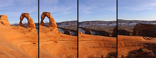
For this project, let us consider a set of sample images with much stronger corners as shown in the Fig. 3.

Fig. 3: Sample image set for panorama stitching

2. Adaptive Non-Maximal Suppression (or ANMS)

The objective of this step is to detect corners such that they are equally distributed across the image in order to avoid weird artifacts in warping. Corners in the image can be detected using cornermetric function with the appropriate parameters. The output is a matrix of corner scores: the higher the score, the higher the probability of that pixel being a corner. Try to visualize the output using the Matlab function imagesc or surf.

To find particular strong corners that are spread across the image, first we need to find $N$_strong corners. Feel free to use MATLAB function imregionalmax. Because, when you take a real image, the corner is never perfectly sharp, each corner might get a lot of hits out of the $N$ strong corners - we want to choose only the $N$_best best corners after ANMS. In essence, you will get a lot more corners than you should! ANMS will try to find corners which are local maxima.

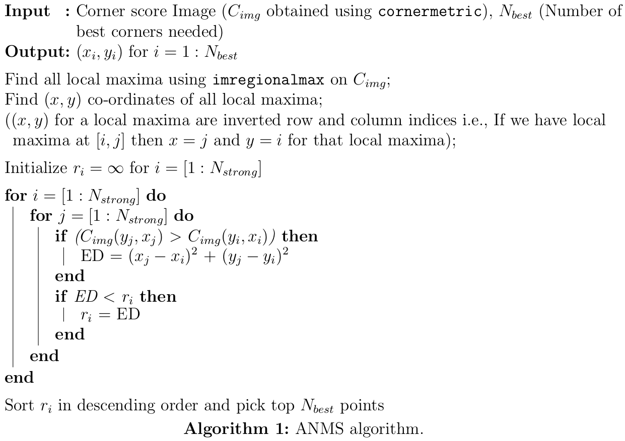
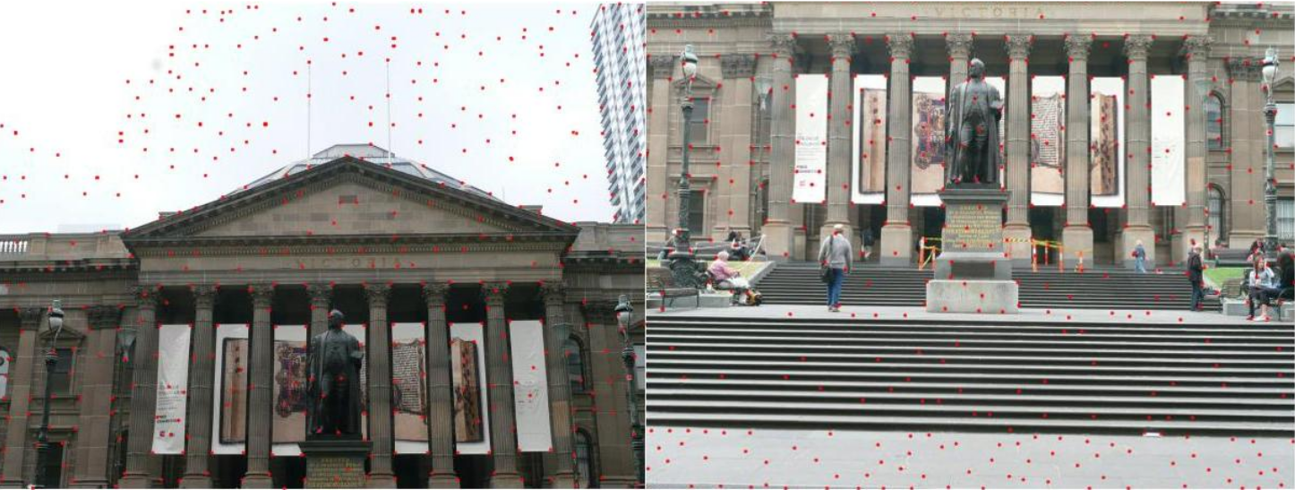
Fig 4. shows the output after ANMS. Clearly, the corners are spread across the image. To plot these dots over the image in MATLAB, do: $\texttt{imshow(..); hold on; plot(...); hold off;}$

Fig. 4: Output of ANMS on first 2 images.

3. Feature Descriptor

In the previous step, you found the feature points (locations of the N best best corners after ANMS are called the feature points). You need to describe each feature point by a feature vector, this is like encoding the information at each feature points by a vector. One of the easiest feature descriptor is described next.

Take a patch of size $40 \times 40$ centered (this is very important) around the keypoint. Now apply gaussian blur (feel free to play around with the parameters, for a start you can use Matlab’s default parameters in fspecial command, Yes! you are allowed to use fspecial command in this project). Now, sub-sample the blurred output (this reduces the dimension) to $8 \times 8$. Then reshape to obtain a $64 \times 1$ vector. Standardize the vector to have zero mean and variance of 1 (This can be done by subtracting all values by mean and then dividing by the standard deviation). Standardization is used to remove bias and some illumination effect.

4. Feature Matching

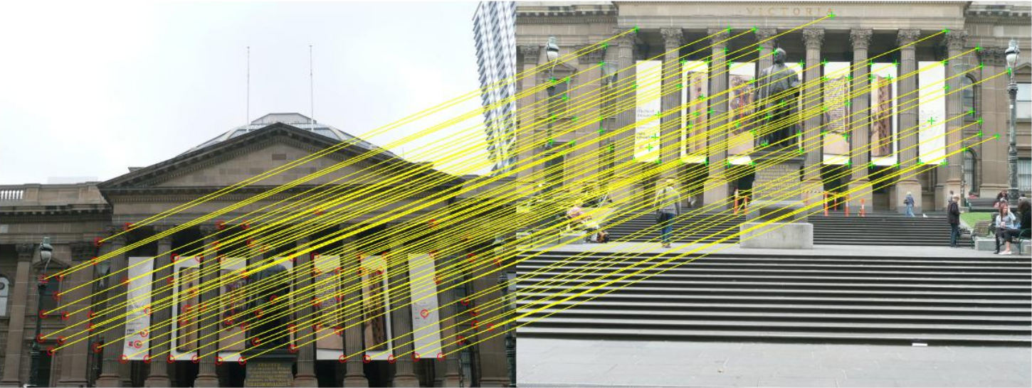
In the previous step, you encoded each keypoint by a $64\times1$ feature vector. Now, you want to match the feature points in the two images so you can stitch the images together. In computer vision terms, this step is referred to as finding feature correspondences within the 2 images. Pick a point in image 1, compute the sum of square difference between all points in image 2. Take the ratio of best match (lowest distance) to the second best match (second lowest distance) and if this is below some ratio keep the matched pair otherwise reject it. Repeat this for all points in image 1. You will be left with only the confident feature correspondences and these points will be used to estimate the transformation between the 2 images also called as Homography. Use the function dispMatchedFeatures given to you to visualize feature correspondences. Fig. 5 shows a sample output of disMatchedFeatures on the first two images.

Fig. 5: Output of \(\texttt{dispMatchedFeatures}\) on first 2 images.

5. RANSAC to estimate Robust Homography

We now have matched all the features correspondences but not all matches will be right. To remove incorrect matches, we will use a robust method called Random Sampling Concensus or RANSAC to compute the homography.

Recall the RANSAC steps are:

1. Select four feature pairs (at random), $p_i$ from image 1, $p_i^1$ from image 2.
2. Compute homography $H$ (exact). Use the function est_homography that will be provided to you. Check Panorama assignment!
3. Compute inliers where $SSD(p_i^1, Hp_i) < \texttt{thresh}$. Here, $Hp_i$ computed using the $\texttt{apply_homography}$ function given to you. $SSD$: Sum of Square Distance.
4. Repeat the last three steps until you have exhausted $N$_max number of iterations (specified by user) or you found more than percentage of inliers (Say $90\%$ for example).
5. Keep largest set of inliers.
6. Re-compute least-squares $\hat{H}$ estimate on all of the inliers. Use the function est_homography given to you.

6. Cylinderical Projection

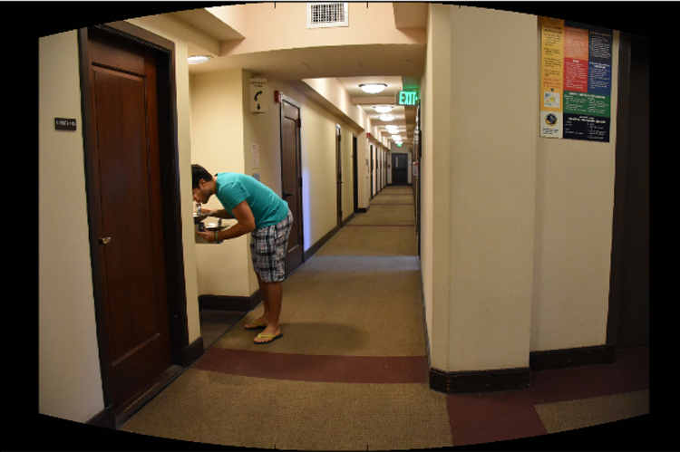
When we are try to stitch a lot of images with translation, a simple projective transformation (homography) will produce substandard results and the images will be strectched/shrunken to a large extent over the edges. Fig. 6 below highlights the stitching with bad distortion at the edges. Check this implementation/demo of cylinderical projection from Stanford Computer Graphics department.

Fig. 6: Panorama stitched using projective transform showing bad distortion at edges.

To overcome such distortion problem at the edges, we will be using cylinderical projection on the images first before performing other operations. Essentially, this is a pre-processing step. The following equations transform between normal image co-ordinates and cylinderical co-ordinates:

In the above equations, $f$ is the focal length of the lens in pixels (feel free to experiment with values, generally values range from 100 to 500, however this totally depends on the camera and can lie outside this range). The original image co-ordinates are $(x, y)$ and the transformed image co-ordinates (in cylindrical co-ordinates) are $(x' ,y')$. $x_c$ and $y_c$ are the image center co-ordinates. Note that, $x$ is the column number and $y$ is the row number in MATLAB.

Note: Use `meshgrid`, `ind2sub`, `sub2ind` to speed up this part. Using loops will TAKE FOREVER!

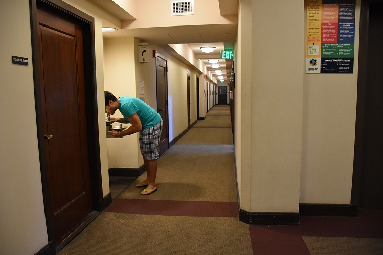
A sample input image and its cylinderical projection is shown in Fig. 7.

Fig. 7: Original Image vs Cylinderical Projection.

Note: The above equations talk about pixel coordinates, NOT pixel values. The idea is you compute the coordinate transformation and copy poaste pixel values to these new pixel coordinates (in all 3 RGB channel).

However, when you compute the values of $(x',y')$ they might not be integers. A simple way to get around this is to use round or actually interpolate the values. If you decide to round the co-ordinates off you might be left with black pixels, fill them using some weighted combination of it’s neighbours (gaussian works best). A trivial way to do this is to blur the image and copy paste pixel values on-to original image where there were pure black pixels. (You can also initialize pixels to NaN’s instead of zeros to avoid removing actual zero pixels).

7. Blending Images:

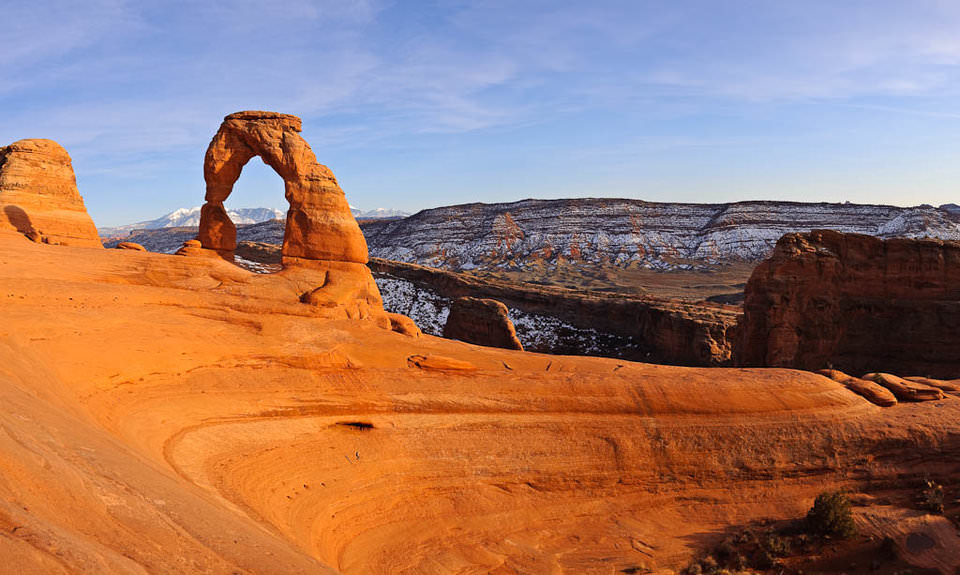
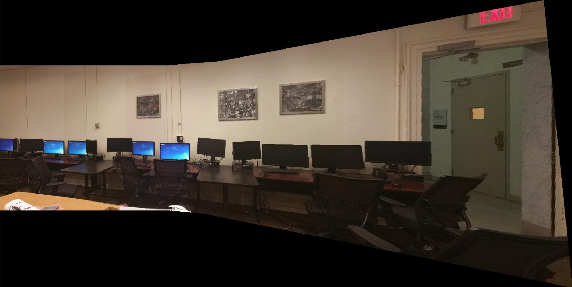
Panorama can be produced by overlaying the pairwise aligned images to create the final output image. The following MATLAB functions can be useful to solve this (like $\texttt{imtransform}$ and $\texttt{imwarp}$). Feel free to implement $\texttt{imwarp}$ or similar function by yourself. For such implementation, apply bilinear tranpolation when you copy pixel values. Feel free to use any third party code for warping and transforming images. Fig. 8 shows the panorama output for the image set in Fig. 3.

Fig. 8: Final Panorama output.

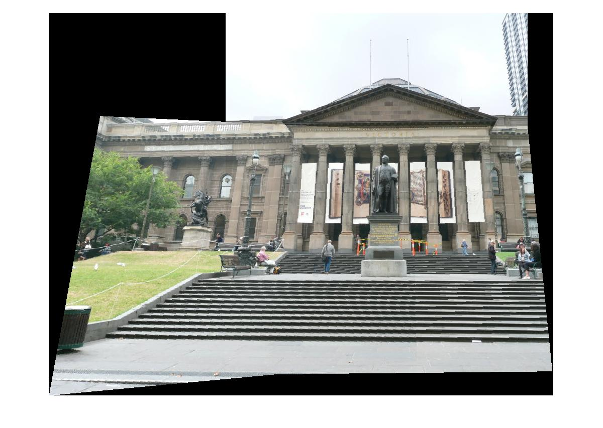
Come up with a logic to blend the common region between images while not affecting the regions which are not common. Here, common means shared region, i.e., a part of first image and part of second image should overlap in the output panorama. Describe what you did in your report. Feel free to use any built-in Matlab function or third party code to do this.

Note: The pipeline talks about how to stitch a pair of images, you need to extend this to work for multiple images. You can re-run your images pairwise or do something smarter.

Your end goal is to be able to stitch any number of given images - maybe 2 or 3 or 4 or 100, your algorithm should work. If a random image with no matches are given, your algorithm needs to report an error.

Note: When blending these images, there are inconsistency between pixels from different input images due to different exposure/white balance settings or photometric distortions or vignetting. This can be resolved by Poisson blending. You can use third party code for the seamless panorama stitching.