Learning the basics of Computer Vision

This article is written by Chahat Deep Singh. (chahat[at]terpmail.umd.edu)

Please contact Chahat if there are any errors.

Table of Contents:

Introduction
Features and Convolution

1. Introduction

We have seen fascinating things that our camera applications like instagram, snachat or your default phone app do. It can be creating a full structure of your face for facial recognition or simply creating a panorama from multiple images. In this course, we will learn how to recreate such applications but before that we require to learn about the basics like filtering, features, camera models and transformations. This article is all about laying down the groundwork for the aforementioned applications. Let’s start with understanding the most basic aspects of an image: features.

2. Features and Convolution

2.1 What are features?

What are features in Machine vision? Is it similar as Human visual perception? This question can have different answers but one thing is certain that feature detection is an imperative building block for a variety of computer vision applications. We all have seen Panorama Stitching in our smartphones or other softwares like Adobe Photoshop or AutoPano Pro. The fundamental idea in such softwares is to align two or more images before seamlessly stitching into a panorama image. Now back to the question, what kind of features should be detected before the alignment? Can you think of a few types of features?

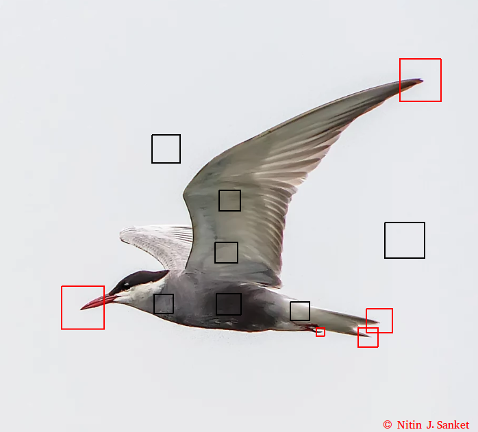
Certain locations in the images like corners of a building or mountain peaks can be considered as features. These kinds of localized features are known as corners or keypoints or interest points and are widely used in different applications. These are characterized by the appearance of neigborhood pixels surrounding the point (or local patches). Fig. 1 demonstrates strong and weak corner features.

Fig. 1: The section in red illustrates good or strong corner features while the black depicts weak or bad features.

The other kind of feature is based on the orientation and local appearance and is generally a good indicator of object boundaries and occlusion events. (Occlusion means that there is something in the field of view of the camera but due to some sensor/optical property or some other scenario, you can’t.) There are multiple ways to detect certain features. One of the way is convolution.

2.2 Convolution

Ever heard of Convolutional Neural Networks (CNN)? What is convolution? Is it really that ‘convoluted’? Let’s try to answer such questions but before that let’s understand what convolution really means! Think of it as an operation of changing the pixel values to a new set of values based on the values of the nearby pixels. Didn’t get the gist of it? Don’t worry!

Convolution is an operation between two functions, resulting in another function that depicts how the shape of first function is modified by the second function. The convolution of two functions, say $f$ and $g$ is written is $f\star g$ or $f*g$ and is defined as:

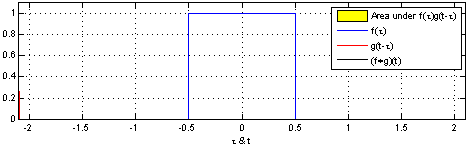
$(f*g)(t) = \int_{-\infty}^{\infty} f(\tau)g(t-\tau)d\tau = \int_{-\infty}^{\infty} f(t-\tau)g(\tau)d\tau$

Let’s try to visualize convolution in one dimension. The following figure depcits the convolution (in black) of the two functions (blue and red). One can think convolution as the common area under the functions $f$ and $g$ .

Convolution of $f$ and $g$ is given by the area under the black curve.

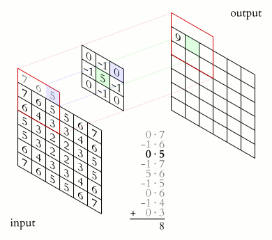
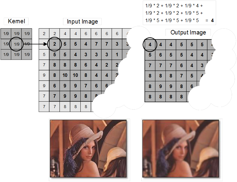
Since we would be dealing with discrete functions in this course (as images are of the size $M\times N$ ), let us look at a simple discrete 1D example: $f = [10, 50, 60, 10, 20, 40, 30]$ and $g = [1/3, 1/3, 1/3]$ . Let the output be denoted by $h$ . What would be the value of $h(3)$ ? In order to compute this, we slide $g$ so that it is centered around $f(3)$ i.e. $\begin{bmatrix}10 & 50 & 60 & 10 & 20 & 40 & 30\\0 & 1/3 & 1/3 & 1/3 & 0 & 0 & 0\end{bmatrix}$ . We multiply the corresponding values of $f$ and $g$ and then add up the products i.e. $h(3)=\dfrac{1}{3}50+\dfrac{1}{3}60\dfrac{1}{3}10=40$ It can be inferred that the function $g$ (also known as kernel or the filter) is computing a windowed average of the image.

Similarly, one can compute 2D convolutions (and hence any $N$ dimensions convolution) as shown in image below:

Convolution of a Matrix with a kernal.

These convolutions are the most commonly used operations for smoothing and sharpening tasks. Look at the example down below:

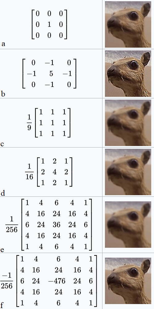
Smoothing/Blurring using Convolution.

Different kernels (or convolution masks) can be used to perform different level of sharpness:

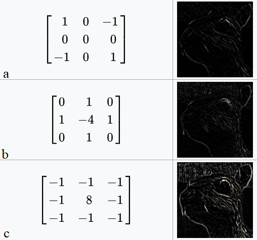
(a). Convolution with an identity masks results the same image as the input image. (b). Sharpening the image. (c). Normalization (or box blur). (d). 3X3 Gaussian blur. (e). 5X5 Gaussian blur. (f). 5X5 unsharp mask, it is based on the gaussian blur. NOTE: The denominator outside all the matrices are used to normalize the operation.

Apart from the smoothness operations, convolutions can be used to detect features such as edges as well. The figure given below shows how different kernel can be used to find the edges in an image using convolution.

Detecting edges in an image with different kernels.

A good explanation of convolution can also be found here.

Deconvolution:

Clearly as the name suggests, deconvolution is simply a process that reverses the effects of convolution on the given information. Deconvolution is implemented (generally) by computing the Fourier Transform of the signal $h$ and the transfer function $g$ (where $h=f * g$ ). In frequency domain, (assuming no noise) we can say that: $F=H/G$ . Fourier Transformation: Optional Read, Video

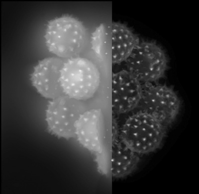
One can perform deblurring and restoration tasks using deconvolution as shown in figure:

Left half of the image represents the input image. Right half represents the image after deconvolution.

Now, since we have learned the fundamentals about convolution and deconvolution, let’s dig deep into Kernels or point operators). One can apply small convolution filters of size $2\times2$ or $3\times3$ or so on. These can be Sobel, Roberts, Prewitt, Laplacian operators etc. We’ll learn about them in a while. Operators like these are a good approximation of the derivates in an image. While for a better texture analysis in an image, larger masks like Gabor filters are used. But what does it mean to take the derivative of an image? The derivative or the gradient of an image is defined as: $\nabla f=\left[\dfrac{\delta f}{\delta x}, \dfrac{\delta f}{\delta y}\right]$ It is important to note that the gradient of an image points towards the direction in which the intensity changes at the highest rate and thus the direction is given by: $\theta=tan^{-1}\left(\dfrac{\delta f}{\delta y}\Bigg{/}\dfrac{\delta f}{\delta x}\right)$ Moreover, the gradient direction is always perpendicular to the edge and the edge strength can by given by: $||\nabla f|| = \sqrt{\left(\dfrac{\delta f}{\delta x}\right)^2 + \left(\dfrac{\delta f}{\delta y}\right)^2}$ . In practice, the partial derivatives can be written (in discrete form) as the different of values between consecutive pixels i.e. 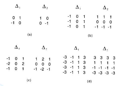$f(x+1,y) - f(x,y)$ as $\delta x$ and $f(x,y+1) - f(x,y)$ as $\delta y$ .

Figure below shows commonly used gradient operators.

Commonly used gradient operators.

You can implement the following in MATLAB using the function edge with various methods for edge detection. Before reading any further, try the following in MATLAB:

C = conv2(A, B) Refer
BW = edge(I, method, threshold, sigma) Refer
B = imfilter(A, h, 'conv') Refer

Different Operators:

Sobel Operator:

This operator has two $3\times 3$ kernels that are convolved with the original image I in order to compute the approximations of the derivatives. The horizontal and vertical are defined as follows:

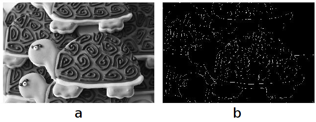
$G_x = \begin{bmatrix} +1 & 0 & -1 \\ +2 & 0 & -2 \\ +1 & 0 & -1 \end{bmatrix}$ $G_y = \begin{bmatrix} +1 & +2 & +1 \\ 0 & 0 & 0 \\ -1 & -2 & -1 \end{bmatrix}$

The gradient magnitude can be given as: $G=\sqrt{G^2_x + G^2_y}$ and the gradient direction can be written as: $\theta=a tan \Bigg(\cfrac{G_y}{G_x}\Bigg)$ . Figure below shows the input image and its output after convolving with Sobel operator.

(a). Input Image. (b). Sobel Output.

Prewitt:

$G_x = \begin{bmatrix} +1 & 0 & -1 \\ +1 & 0 & -1 \\ +1 & 0 & -1 \end{bmatrix}$ $G_y = \begin{bmatrix} +1 & +1 & +1 \\ 0 & 0 & 0 \\ -1 & -1 & -1 \end{bmatrix}$

Roberts:

$G_x = \begin{bmatrix} +1 & 0 \\ 0 & -1 \end{bmatrix}$ $G_x = \begin{bmatrix} 0 & +1 \\ -1 & 0 \end{bmatrix}$

Canny:

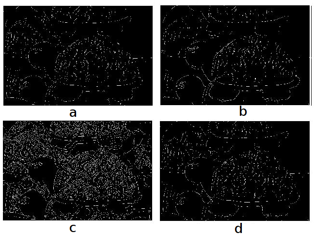
Unlike any other filters, we have studied above, canny goes a bit further. In Canny edge detection, before finding the intensities of the image, a gaussian filter is applied to smooth the image in order to remove the noise. Now, one the gradient intensity is computed on the imge, it uses non-maximum suppression to suppress only the weaker edges in the image. Refer: A computational approach to edge detection. MATLAB has an approxcanny function that finds the edges using an approximate version which provides faster execution time at the expense of less precise detection. Figure below illustrates different edge detectors.

(a). Prewitt Output. (b). Roberts Output. (c). Canny Output (d) Laplacian of Gaussian (LoG).

Corner Detection:

Now that we have learned about different edge features, let’s understand what corner features are! Corner detection is used to extract certain kinds of features and common in panorama stitching (Project 1), video tracking (project 3), object recognition, motion detection etc.

What is a corner? To put it simply, a corner is the intersection of two edges. One can also define corner as: if there exist a point in an image such that there are two defintive (and different) edge directions in a local neighborhood of that point, then it is considered as a corner feature. In computer vision, corners are commonly written as ‘interest points’ in literature.

The paramount property of a corner detector is the ability to detect the same corner in multiple images under different translation, rotation, lighting etc. The simplest approach for corner detection in images is using correlation. (Correlation is similar in nature to convolution of two functions). Optional Read: Correlation

In MATLAB, try the following:

corner(I, 'detectHarrisFeatures'): Harris Corners
corner(I, 'detectMinEigenFeatures'): Shi-Tomasi Corners
detectFASTFeatures(I): FAST: Features from Accelerated Segment Test

Harris Corner Detection.