Math Tutorial

This article is written by Nitin J. Sanket.

updated by Cornelia Fermüller (1/21/2019)

The Table of Contents:

Hilbert Space, Vectors, Dot and Cross Products
Eigenvalues and Eigenvectors
Singular Value Decomposition (SVD)
Line fitting using Linear Least Squares
- Null-space
$A\mathbf{x}=\mathbf{b}$
Effect of outliers on $A\mathbf{x}=\mathbf{b}$ and Regularization to combat them
Random Sample Consensus (RANSAC) for outlier rejection

Hilbert Space, Vectors, Dot and Cross Products

In the simplest sense, the Euclidean space we consider in everyday life is mathematically called the Hilbert Space. The co-ordinates of the Hilbert space can represent anything from physical metric coordinates (most general sense) to something like the cost of goods, the volume of goods and so on. Any general metric graph is a Hilbert Space. An $n$ dimensional Hilbert space is said to live in $\mathbb{R}^n$ which indicates that all the numbers represented in this space are real. Note that Cartesian space is different from Hilbert space and is a sub-set of it. Mathematically, a Hilbert space is an abstract vector space which preserves the structure of an inner product. In non-math terms, it just means that one can measure length and angle in this space.

Now, for the sake of easy discussion and without loss of any generality let us assume that our Hilbert Space is in $\mathbb{R}^3$. Think of this as our $X-Y-Z$ coordinate space. Any point in space $p$ is represented as a triplet $[x,y,z]^T$, i.e., having three values (one for the x-coordinate, one for the y-coordinate and one for the z-coordinate). I made an implicit assumption when I said that we have an $X-Y-Z$ coordinate space. Can you think of what it is?

Simply, I assumed that the three axes (basis) are perpendicular or orthogonal to each other. One may ask why we need this condition? This is to have the minimal amount of values to represent any data in the space and to have a unique combination of these axes (basis) to represent a point. Also, the axes are represented by unit vectors for representing direction only (more about this later). Now any point in the space represents a vector from the origin $[0,0,0]^T$ to itself, i.e., the tail of the vector is at the origin and the head of the vector is at the point. Note that the vector is a column vector. This is the general mathematical representation of a vector. Otherwise unless stated, vectors are assumed to be column vectors.

Now let us assume that the space is Cartesian. One might wonder what other spaces exist? Think of cylindrical coordinates or spherical coordinates which are used in panorama stitching on your phone for Virtual Reality. Let us assume that we have three points in this space denoted as $A, B, C$. The vector from the origin to either $A$ or $B$ or $C$ is denoted by their respective coordinates. Now a vector between two points $A, B$ is represented as $\vec{AB}$ and is given by $\vec{AB} = B - A$.

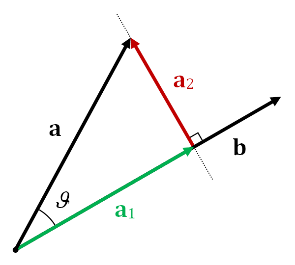
The dot product between two vectors $ \vec{AB}, \vec{BC} $ is defined as $ \vec{AB}\cdot \vec{BC} = \vert \vert \vec{AB} \vert \vert \vert \vert \vec{BC} \vert \vert \cos \theta$. Here, $\vert \vert \vec{AB} \vert $\vert represents norm of the vector $\vec{AB}$ and is given as $ \sqrt{AB_x^2 + AB_y^2 + AB_z^2}$, where $\vec{AB} = [AB_x, AB_y, AB_z]^T$. $ \theta $ is the angle between the two vectors. Note that the dot product is a scalar value. The dot product represents the projection of one vector onto another vector. This is generally used to measure similarity of vectors in Computer Vision, such as for example in processing 3D data from multiple cameras or from a Kinect sensor. Note that the dot product is commutative ($\mathbf{a}\cdot \mathbf{b} = \mathbf{b}\cdot \mathbf{a}$) and not associative because the dot product between a scalar ($a \cdot b$) and a vector ($c$) is not defined. $(a \cdot b) \cdot c$ or $a \cdot (b \cdot c$) are both ill-defined. Other properties can be found here.

Projection of $a$ on $b$ ($a1$), and subtraction of $a$ from $b$ ($a2$).

It is incovinent to write the vector superscript everytime, so a boldface text is commonly used to represent vectors, for eg., $ \vec{AB}$ and $ \mathbf{AB}$ represent the same thing.

The cross product between two vectors $\mathbf{a}, \mathbf{b}$ is defined as $ \mathbf{a} \times \mathbf{b} = \vert \vert \mathbf{a} \vert \vert \vert \vert \mathbf{b} \vert \vert \sin \theta \mathbf{n}$. Here $ \mathbf{n}$ is the vector perpendicular/normal to the plane containing the two vectors $ \mathbf{a}, \mathbf{b} $ and $\theta$ is the angle between the two vectors. The direction of the cross product is found using the right hand rule in a right handed coordinate system.

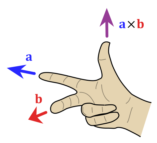
Finding the direction of the cross product by the right-hand rule.

An animation of the cross product is shown below:

The cross product $ \mathbf{a} \times \mathbf{b}$ (vertical, in purple) changes as the angle between the vectors $ \mathbf{a} $ (blue) and $ \mathbf{b} $ (red) changes. The cross product is always orthogonal to both vectors, and has magnitude zero when the vectors are parallel and maximum magnitude $ \vert \vert \mathbf{a} \vert \vert \vert \vert \mathbf{b} \vert \vert $ when they are orthogonal.

The cross product is used to find the normal vector to a plane in Computer Vision. This is especially useful in aligning 3D point clouds (images with depth information). This method is extensively used in self driving cars to make a map using LIDAR scans. If you are curious, have a look at the Point to Plane Iterative Closest Point algorithm to understand how this works. Note that the cross prodct is anticommutative ($\mathbf{a}\times \mathbf{b} = -\mathbf{b}\times\mathbf{a}$) and not associative. Other properties can be found here.

Eigenvalues and Eigenvectors

In the following we consider transformations with square matrices (i.e. the matrix $ A \in \mathbb{R}^{n \times n}$), and which are diagonizable, such as the symmetric matrices of the covariance of data.

Let us say we have a vector $\mathbf{v}$ in $ \mathbb{R}^n$. A linear transformation of $\mathbf{v}$ is given by a matrix $A$ multiplied by $\mathbf{v}$. One could have a special vector $\mathbf{v}$ such that the function $A \mathbf{v}$ returns a scaled version of $\mathbf{v}$, i.e., the direction of the $ \mathbf{v}$ is maintained upon a linear transformation by $A$. This can mathematically be written as:

$A \mathbf{v} = \lambda \mathbf{v}$

Note that $ \lambda \mathbf{v}$ is a scaled version of $\mathbf{v}$, i.e., the direction of both the vectors is the same. Recall, that the direction of a vector $\mathbf{v}$ is given by $\frac{\mathbf{v}}{\vert \vert \mathbf{v} \vert \vert}$. The concept of scale factor is very important for computer vision and will be later used in the last project.

In the above transformation $ A \in \mathbb{R}^{n \times n}$. Now one can solve the above equation as follows:

$\left(A - \lambda I \right)\mathbf{v} = 0$

Here $ I$ is an identity matrix of size $ n \times n$ and has all the diagonal elements as 1 and non-diagonal elements as 0. Once the above equation is solved, one would find $n$ pairs of $\lambda_i$ and $\mathbf{v}_i$ such that the above equation is satisfied ($i$ varies from 1 to $N$). These set of $\lambda_i$ values are called eigenvalues and these set of $\mathbf{v}_i$ vectors are called eigenvectors. Note that the eigenvectors are linearly independent, i.e., the dot product between any of them is zero. However, the eigenvalues need not be distinct if we have a matrix $Q$ whose columns are made up of the eigenvectors, i.e.,

$Q = \begin{bmatrix} \mathbf{v_1} & \mathbf{v_2} & \cdots & \mathbf{v_n} \end{bmatrix}$

Now, consider $ AQ$ and the fact that $ A \mathbf{v} = \lambda \mathbf{v}$.

$AQ = \begin{bmatrix} \lambda_1\mathbf{v_1} & \lambda_2\mathbf{v_2} & \cdots & \lambda_n\mathbf{v_n} \end{bmatrix}$

This can be re-written as:

$AQ = \begin{bmatrix} \mathbf{v_1} & \mathbf{v_2} & \cdots & \mathbf{v_n} \end{bmatrix} \Lambda$

Here $\Lambda$ is a diagonal matrix with $\Lambda_{ii} = \lambda_i$. We also know that the columns of $Q$ are linearly independent, and this means that $Q$ is invertible.

$A = Q\Lambda Q^{-1}$

The above is called Eigen-decomposition in the literature. Eigen-decomposition is very commonly used in an algorithm called Principle Component Analysis (PCA). PCA is used to find the most important linearly independent basis of a given data.

You might be wondering what the intuition to Eigen-decomposition is. The eigenvalues represent the covariance and eigenvectors represent the linearly independent directions of variation in data. Sample eigenvectors and eigenvalues are shown below:

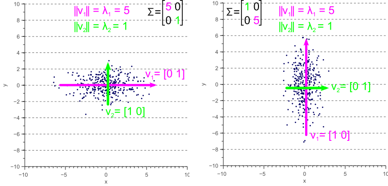
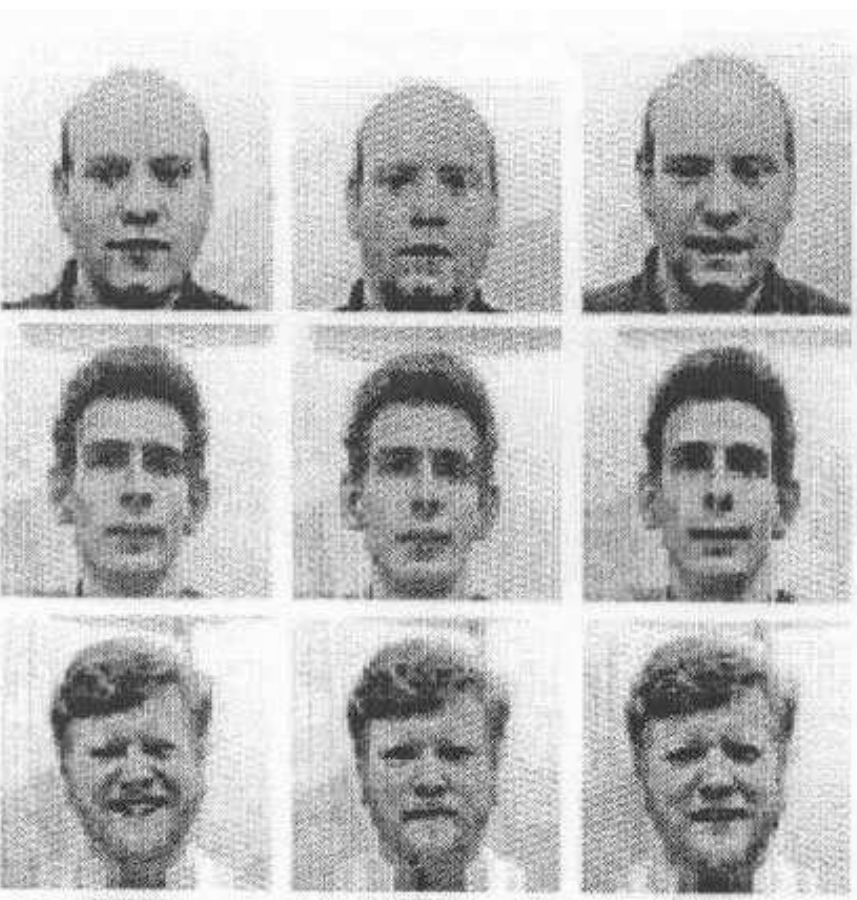
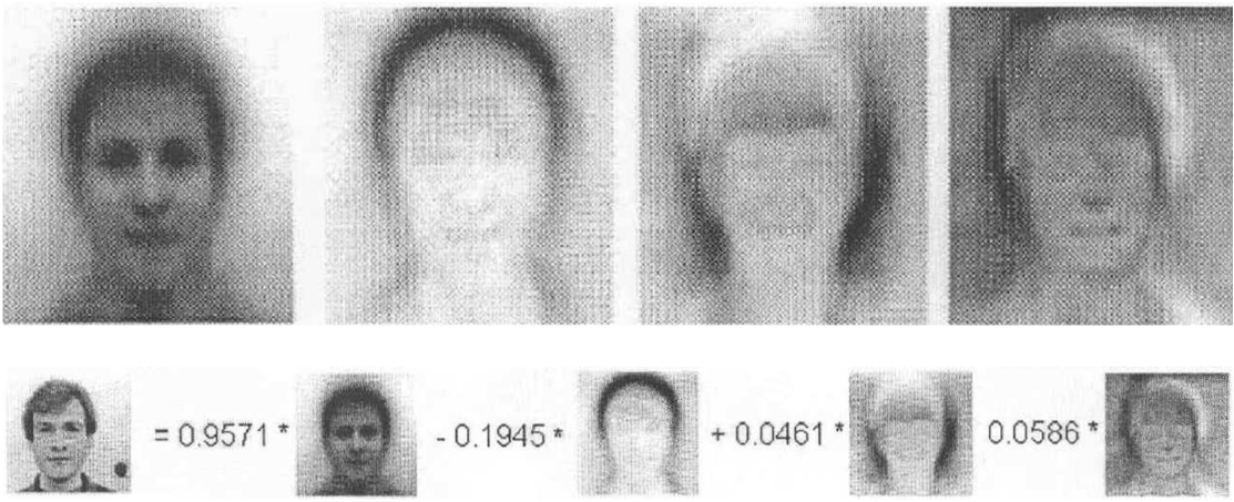
Eigenvectors of a covariance matrix of data shown in blue. Data is drawn from a gaussian distribution.

For a detailed explanation of the visualization look at this link. In computer vision, eigenspaces have been used for ages. Consider the problem of face recognition. Here we have a dataset of a lot of faces and we need to identify the person given a photo of the face. This is similar to what TSA does when they check your ID at the airport, they are manually trying to see if the photo in the ID looks like the person in front of them. One of the earliest face recognition methods used eigenspaces and the algorithm is aptly called Eigenfaces. The idea of the algorithm is to represent any face as a linear combination of eigenfaces. These eigenfaces are supposed to represent the most common features of a face and that any face can be reconstructed as their linear combination. This means that each face is represented as a vector of weights which multiply these eigenfaces and are added up to make the original face. Think of this as representing each face as an encoded vector. This idea is also used extensively in compression. During the face identification, the test face is also converted to a vector and the label (person ID) of closest vector in the training set (database of face images on the computer) is chosen as the predicted label (person ID). A visual representation of this is shown below. For more details look at this link.

Sample images in the database/training set.

Top row: Eigenfaces. Bottom row: How any face can be represented as a linear combination of eigenfaces.

Note that Eigendecomposition only works on square matrices.

Singular Value Decomposition (SVD)

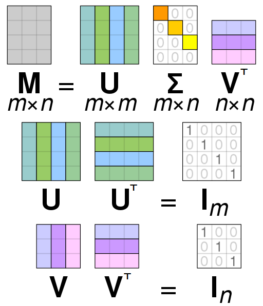
One can think of SVD as the generalized version of the Eigen-decomposition. Let $ A$ be a matrix of size $m \times n$. The SVD of $A$ is given by:

$A = U\Sigma V^T$

Note that $\Sigma$ here does not refer to the covariance matrix. Here, $U$ is a $m \times m$ square orthonormal basis function. The columns of $U$ form a set of orthonormal (unit normal) vectors which can be regarded as basis vectors. $V^T$ is a $n \times n$ square orthonormal basis function as well. The columns of $V$ also form a set of orthonormal (unit normal) vectors which can be regarded as basis vectors. Think of $U, V^T$ as matrices which rotate the data. $\Sigma$ is a $m \times n $ diagonal rectangular matrix which acts as a scaling matrix. Note that for SVD to be valid $A $ has to be a Positive Semi-Definite matrix (PSD), i.e., $ A \succeq 0$ or all the eigenvalues have to be non-negative (either zero or positive). You might be wondering this looks very similar to the eigendecomposition we studied earlier. What is the relation between the two?

The matrix $U$ (left singular values) of $A$ gives us the eigenvectors of $AA^T$. Similarly, as you expect, the matrix $V$ (right singular values) of $A$ gives us the eigenvectors of $A^TA$. The non-zero singular values of $A$ (found on diagonal entries of $\Sigma$) are the square roots of non-zero eigenvalues of both $AA^T$ and $A^TA$.

Visualization of the matrix multiplications in singular value decomposition.

Visualization of how different components of SVD make up the matrix $A$.

Line fitting using Linear Least Squares

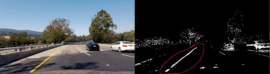
Let us define the problem in hand first. Assume that we have $N$ points in $\mathbb{R}^n$, for purposes of simplicity without loss in any generality let $n=2$. We want to fit a line (the equivalent is a plane in $\mathbb{R}^n$ and a hyperplane in $\mathbb{R}^n$). When $N = 1$, one can fit $\infty$ number of lines which satisfy the constraint of passing though the point and hence has no unique exact (the line passes through the point) solution. Now, when $N = 2$, one can fit a unique and exact solution because we have exactly the same number of parameters (number of unknowns in the line equation) as the number of constraints (equations). However, things get tricky when $N > 2$. One might wonder when we would encouter such a situtation, this is more common than you think. Assume that we want to fit a line to a number of pixels in an image, possible to detect a lane on an self driving car.

Left: Input image to a self driving car for lane detection. Right: Pixel candidates where one would fit a line to find the lane, notice that there are multiple lines possible, for the purposes of the example assume that we want to fit a line to the pixels inside the red ellipse.

Let us model the problem mathematically, we have $N$ points in $\mathbb{R}^2$ to which we want to fit the best-fit line. The best-line has to be defined before we proceed. One could argue that I can pick any random two points and fit a line and call that the best-fit. However, this solution is the best for those two points and not for all points. If all the points lie on a line one could say that we have an exact and unique solution, but this rarely happens. The more common version of this problem is that the best-fit line generally would not pass through any of the points. You might be wondering why then is it the best line? Well, it depends on how we are going to define best-fit, and that the points are noisy. Let us define best-fit right now.

Let the equation of the line be $ax+by+c=0$ where we want to find the parameters $\Theta=\begin{bmatrix} a & b & c \end{bmatrix}^T$ such that:

$\underset{\Theta}{\operatorname{argmin}}\sum_{i=1}^N R(x_i,y_i \vert \Theta)^2$

$\underset{\Theta}{\operatorname{argmin}}$ means that we want to minimize and find the parameters $\Theta$ which gives us the minimum value. The function $R$ defines the best-fit here which is what the user has chosen. Let us choose $R$ to be a function which computes the distance (offsets) from any point $[x,y]^T$ to the line $ax+by+c=0$. This can be of two variants, i.e., vertical distances/ offsets and/or perpendicular distance/offsets.

Left: Vertical distances/offsets. Right: Perpendicular distances/offsets.

Because it is more inuitive, let us choose the perpendicular distance/offsets for $R$. The perpendicular distance of any point $[x,y]^T$ to the line $ax+by+c=0$ is given by:

$R(x,y \vert \Theta) = \frac{ax+by+c}{\sqrt{a^2+b^2}}$

So our optimization/minimization problem becomes:

$\underset{\Theta}{\operatorname{argmin}}\sum_{i=1}^N \frac{\left(ax+by+c\right)^2}{a^2+b^2}$

The function $\sum_{i=1}^N \frac{\left(ax+by+c\right)^2}{a^2+b^2}$ depicts the sum of distances (this is just a scaled version of the average) from each point to the line. Because we are minimizing the square of $R$, the minimum value the optimization function can take is 0. This happens when all the points like exactly on the line. Like we said before, this rarely happens and in these cases there is no-exact solution (only some/no points pass through the line). This solution is called the Least-squares solution and the optimization problem is referred to as Ordinary Least Squares (OLS) or Linear Least Squares or Linear Regression in the machine learning community. (In Estimation Theory, the fitting minimizing the perpendicular offsets is also referred to as Total Least Squares Estimation). To find the solution, let us write down the constraints we have. We ideally want all points to lie on the best-fit line. This can mathematically be written as:

$ax_1 + by_1 + c = 0\\ ax_2 + by_2 + c = 0\\ \vdots \\ ax_N + by_N + c = 0\\$

Now let us write this down in matrix form:

$\begin{bmatrix} x_1 & y_1 & 1 \\ & \vdots & \\ x_N & y_N & 1\end{bmatrix} \begin{bmatrix} a \\ b \\c \end{bmatrix} = \mathbf{0}$

The trivial solution to the above problem is obtained when $\begin{bmatrix} a \ b \ c \end{bmatrix}^T = 0$. This is the case where the constraint mathematically satisfies the solution but physically doesn’t make much sense as we get back the origin. To avoid this we modify the optimization problem as follows:

$\begin{equation*} \begin{aligned} & \underset{\Theta}{\text{argmin}} & & \sum_{i=1}^N \frac{\left(ax+by+c\right)^2}{a^2+b^2} \\ & \text{subject to} & & \vert \vert \Theta \vert \vert = 1 \end{aligned} \end{equation*}$

Note that, we haven’t changed anything but just added a constraint saying that the norm of the line equation coefficients should be unity. This avoides the trivial solution gracefully. This optimization problem can be written in matrix form as follows:

$\begin{equation*} \begin{aligned} & & A\Theta = \mathbf{0}\\ & \text{subject to} & \vert \vert \Theta \vert \vert = 1 \end{aligned} \end{equation*}$

Where, $A = \begin{bmatrix} x_1 & y_1 & 1 \\ & \vdots & \\ x_N & y_N & 1\end{bmatrix}$ and $\Theta = \begin{bmatrix} a \\ b \\c \end{bmatrix}$ .

To solve the above optimization problem which is of the form $Ax=0$, we need to understand the concept of Null-space.

Null-space

Null-space or kernel of a linear map $L: V \rightarrow W $ between two vector spaces $V, W$ is the set of all elements such that $L(\mathbf{v})=0$. In set notation,

$\ker(L) = \text{null}(L) = \left\{\mathbf {v} \in V \vert L(\mathbf {v} )=\mathbf {0} \right\}$

To understand how this will help in solving $A\mathbf{x}=0$, we need to understand the concept of rank of a matrix first. The rank of a matrix $A$ is defined as the number of linearly independent columns of $A$, this is mathematically defined as the dimension of the vector space spanned by the columns of $A$. The easiest way to find the rank of a matrix is to take the Eigen-decomposition (for square matrices) or the SVD (for any shaped matrix). The number of non-zero eigenvalues or the number of non-zero singular values gives the rank of a matrix. The rank can be at most the smallest dimension of the matrix $A$, i.e., if $A \in \mathbb{R}^{m \times n}$ and $n < m $ , then $\text{rank}(A)\le n$. Now that we know what rank means, we can state the Rank-nullity theorem as follows:

$\text{rank}(A) + \text{nullity}(A) = n$

This means that a solution of the form $A\mathbf{x}=0$ lies in the null-space of $A$.

Let us find the nullspace using SVD. Let the SVD of $A = U\Sigma V^T$. Now, $\Sigma$ is ideally supposed to be of rank 3 (as we know that we have 3 unknowns). This means that the 4:N rows of $\Sigma$ have to be all zeros. But due to noise, the rank will be more than 3. A good solution to the optimization problem is obtained when we set any of the columns of $V^T$ corresponding to nullspace to zero (4:N rows of $\Sigma$). The singular values are sorted in descending order and hence a minimum deviation from the ideal line would give us the best-fit solution. This is the solution corresponding to the smallest singular-value.

The best-fit solution is therefore given by the last column of $V$ (last row of $V^T$ ).

Note that, a simple assumption made about the noise in the previous line fitting example is that, the noise is white gaussian with a mean of zero and some standard deviation. Inuitively, it means that the probability of data points away from the line is decreases as the distance between the point and the line increases. Mathematically the noise is derived from the following distribution (Co-variance is denoted as $\Sigma$):

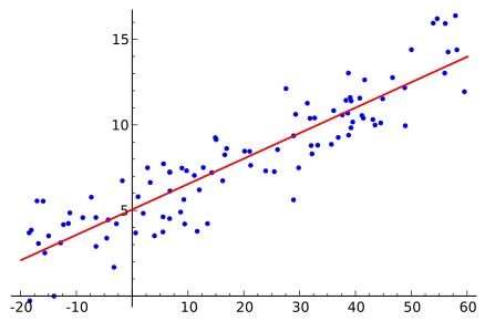
$p(\mathbf{x}) = \frac{1}{\sqrt{(2 \pi)^3 \vert \Sigma \vert}}e^{\left(\frac{1}{2}(\mathbf{x})^T\Sigma^{-1}(x)\right)} = \mathcal{N(\mathbf{x} \vert 0, \Sigma)}$

Here, $\mathbf{x}$ represents the vector in a space $\mathbb{R}^n$. In our line-fitting example, $n=2$. Sample datapoints with their linear least-squares line solution is shown below:

Random data points and their linear least-squares line solution.

$A\mathbf{x}=\mathbf{b}$

You might be wondering what the title means. The last method ($A\mathbf{x}=\mathbf{0}$) we solved is called Linear Homogeneous set of equations and $A\mathbf{x}=\mathbf{b}$ is called Linear Inhomogeneous set of equations. The problem formulation is slightly different from the earlier case as one would except.

We have $N$ observations of $[\mathbf{x_i}, \mathbf{y_i}]^T$ where $x_i \in \mathbb{R}^{n \times 1}$ and $y_i \in \mathbb{R}^1$. We want to fit a model such that

$y_i = \mathbf{x_i}^T \beta$

However due to noise (assumed to be gaussian with mean zero and some co-variance, i.e., ) the data samples are obtained from:

$y_i = \mathbf{x_i}^T \beta + \mathcal{N}(\mathbf{x} \vert 0, \Sigma)$

In matrix form:

$\mathbf{y} = \mathbf{X}^T \beta + \mathcal{N}(\mathbf{x} \vert 0, \Sigma)$

The optimization problem is defined next:

$\begin{equation*} \begin{aligned} & \underset{\beta}{\text{argmin}} & & \vert \vert \mathbf{y} - \mathbf{X}\beta \vert \vert \\ \end{aligned} \end{equation*}$

The Ordinary least squares solution is given by:

$\hat{\beta} = \left( \mathbf{X}^T \mathbf{X}\right)^{-1} \mathbf{X}^T\mathbf{y}$

The matrix $\mathbf{X}^T \mathbf{X} $ is called the Gram matrix and is Positive Semi Definite (PSD) (all eigenvalues $\ge 0$). The matrix $ \mathbf{X}^T\mathbf{y}$ is called the moment matrix. For a detailed derivation look at this blog post. If you don’t remember matrix properties, have a look at The Matrix cookbook.

Effect of outliers on $A\mathbf{x}=\mathbf{b}$ and Regularization to combat them

In the previous section, we only talked about how one could obtain the least squares solution but did not analyze what the effect of noise would be. Let $A $ be a $m \times n$ matrix. Consider the solution to $ A\mathbf{x}=\mathbf{b}$. The solution to this problem would be $ \mathbf{x} = A^\dagger \mathbf{b}$ where $A^\dagger$ denotes the pseudo-inverse of $A$. Computing the pseudo-inverse doesn’t look that trivial, does it? Luckily, we have SVD to the rescue!

If SVD of $A$ is given as $A=U\Sigma V^T$, then $A^\dagger = V\Sigma^{-1}U^T$. Here $\Sigma^{-1}$ is defined such that all the non-zero elements are inverted and zeros are maintained as is. If $\mathbf{b}$ is noisy, we have $b = \hat{b} + \mathcal{N(\mathbf{x} \vert 0, \sigma)}$ where $ \hat{\mathbf{b}} $ is the value without noise. If one tries the reconstruct with a noisy $\mathbf{b}$ the solution $\mathbf{x}$ obtained would be complete junk (or super noisy depending on $A$). Don’t worry you’ll do this in your homework. Why did this happen? All the singular values are affected equally by noise, so the smallest singular value gets affected by a relatively large noise which makes the estimated $\mathbf{x}$ super noisy, i.e., much more noisier than $\mathbf{b}$. In fact, the noise gets amplified by $\Lambda_{ii}^{-1}$ (the inverse of the singular value), this number is huge when the singular value is small. In fact, there is a term which signifies the noise sensitivity of the matrix $A$ and is given by:

$\kappa = \frac{\sigma_{max}}{\sigma_{max}} = \left\lvert\frac{\lambda_{max}}{\lambda_{min}} \right\rvert$

(\kappa) is known as the condition number. Here $\sigma_{max}$ and $\sigma_{min}$ refers to the maximum and minimum singular values respectively. Similarly, $\lambda_{max}$ and $\lambda_{min}$ refers to the maximum and minimum eigenvalues respectively. If the noiseless version of the problem is $\mathbf{\hat{x}} = A^\dagger \mathbf{\hat{b}}$ and the noisy version is $\mathbf{x} = A^\dagger \mathbf{b}$, the relation between the estimates and condition number is given below:

$\frac{\vert \vert \mathbf{x} - \mathbf{\hat{x}}\vert \vert}{\vert \vert\mathbf{\hat{x}}\vert \vert} \le \kappa \frac{\vert \vert \mathbf{\hat{b}} - \mathbf{b}\vert \vert}{\vert \vert\mathbf{\hat{b}}\vert \vert}$

Clearly, one can observe that the noise is amplified by a factor of $\kappa$. A high $\kappa$ can lead to optimization problems to fail and is a huge research topic.

However, years of research has given good insight into the above problem and one of the simplest methods to combat the effect of noise is to modify the optimization problem as follows:

$\begin{equation*} \begin{aligned} & \underset{\beta}{\text{argmin}} & & \vert \vert \mathbf{y} - \mathbf{X}\beta \vert \vert + \lambda \vert \vert \beta \vert \vert^2\\ \end{aligned} \end{equation*}$

In the above problem, $\lambda$ is a user chosen value which determines the amount of penalization/penalty (prior) on the norm of $\beta$. This new optimization problem is called the Ridge Regression or Tikhonov regularization or Linear least squares with L$_2$ penalty. As you would expect, this also has a closed form solution given by:

$\hat{\beta} = \left( \mathbf{X}^T \mathbf{X} + \lambda I \right)^{-1} \mathbf{X}^T\mathbf{y}$

Here, $I$ is the identity matrix. The reason why Ridge regression can handle noise better than linear regression is that it improves the condition number of $ \mathbf{X}^T \mathbf{X} $. The new condition number becomes $ \frac{\sigma_{max}^2 + \lambda}{\sigma_{min}^2 + \lambda}$. This value is lower than the original condition number we had which means that the solution is less sensitive to noise. This is similar to adding prior information to the optimization problem which acts as a noise removal filter. In Bayesian terms, this is finding the Maximum a-posteriori (MAP) estimate for the Gaussian noise assumption.

Random Sample Consensus (RANSAC) for outlier rejection

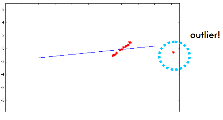
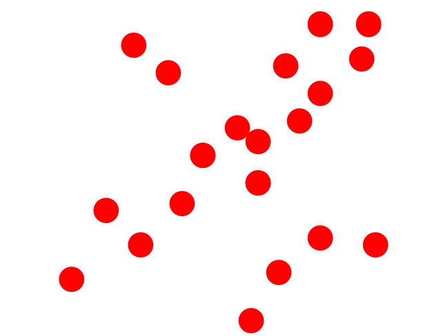
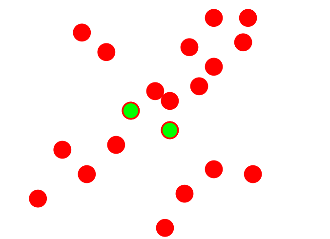
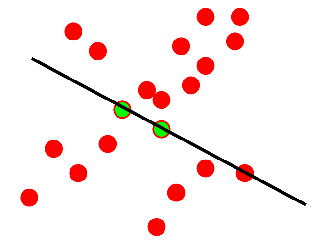
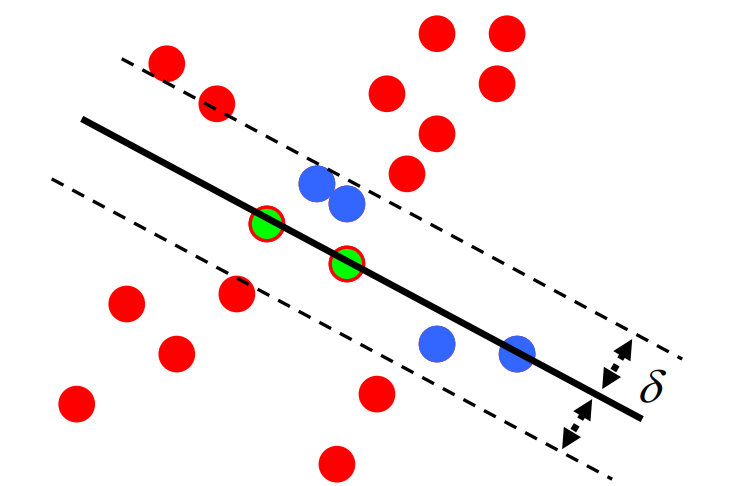
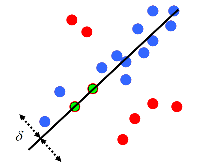
All the above methods work well for noise but not for outliers. The outliers shift the result in the direction of the outliers (see figure below).

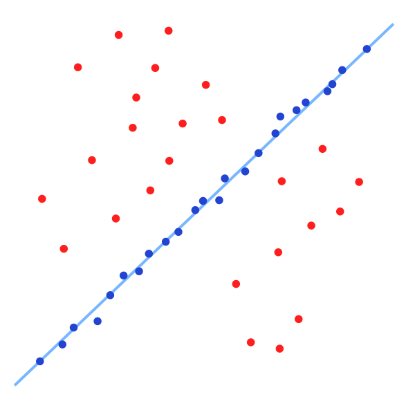
Fitted line is heavily affected by outliers.

The image below shows what we want RANSAC to do. The red points show the points excluded as outliers for solving the line fitting problem. The blue points are the points included in the line fitting solution. The blue line shows the fitted line without outliers.

Fitted line with RANSAC. Observe that outliers have no influence on the result.

The idea of RANSAC is voting. RANSAC makes the following assumptions:

Assumption 1: Noise features will not vote consistently for any single model (“few” outliers when compared to inliers).

Assumption 2: There are enough features to agree on a good model (“few” missing data).

RANSAC algorithm is very simple and can be implemented in less than 40 lines in MATLAB. The algorithm is as follows:

Step 1: Select random sample of minimum required size to fit model (in our case 2, a minimum of 2 points are required to fit a line).

Step 2: Fit the best model from sample set (line passing through both points).

Step 3: Compute the set of inliers to this model from whole data set (inliers are defined as those points whose distance to the fitted line are less than some user chosen threshold).

Repeat Steps 1-3 until model with the most inliers over all samples is found (or for some set number of iterations or until an inlier set is a certain percentage of the data, like 90%).

All the data points given. We want to ignore the outliers and fit a least squares line.

Select 2 points at random.

Fit a line to the selected 2 points.

Measure number of inliers. Here we have 4 inliers.

Repeat steps 1-3. Here we have 12 inliers. These awesome figures are adapted from Prof. Silvo Savarese's slides.

The number of iterations $N$ needed to have a probability $p$ of success with 2 points being chosen at every iteration to fit a line and at an outlier ratio $e$ chosen at each step is given by

$N = \frac{\log\left(1-p\right)}{\log\left(1-\left( 1 - e\right)^2 \right)}$

To put this in perspective, we only need 17 iterations to be 95% sure that we’ll find a good solution even with 50% outliers.

Another voting scheme which works well for fitting curves with a smaller number of parameters is the Hough Transform. This is left as a self-reading article.