Written by Jack Rasiel

• Note: These course notes accompany Project 3. See the Project 3 prompt for details on that assigment.

Segmentation with Fixations

Table of Contents:

• Introduction
• Graph-based Segmentation: a Toy Example
• Fixation-based Segmentation
• Adding Additional Image Features
• Recap
• Appendix

Introduction

For this project, we’ll explore one way to approach image segmentation.

Segmentation is a fundamental problem in computer vision: given an image, how do we partition it into a set of meaningful regions? This definition is intentionally vague (what defines a “meaningful region”?), as there are many different sub-problems which are referred to as “segmentation”. We may be interested in partitioning an image such that every region has a distinctive category, or simply partitioning an image into a foreground region (containing an object of interest) and a background region (containing everything else).

Segmentation into categories. Image from Mishra, Ajay K., and Yiannis Aloimonos. "Visual segmentation of “Simple” objects for robots." *Robotics: Science and Systems VII* 217 (2012).

Source: Wikimedia Commons

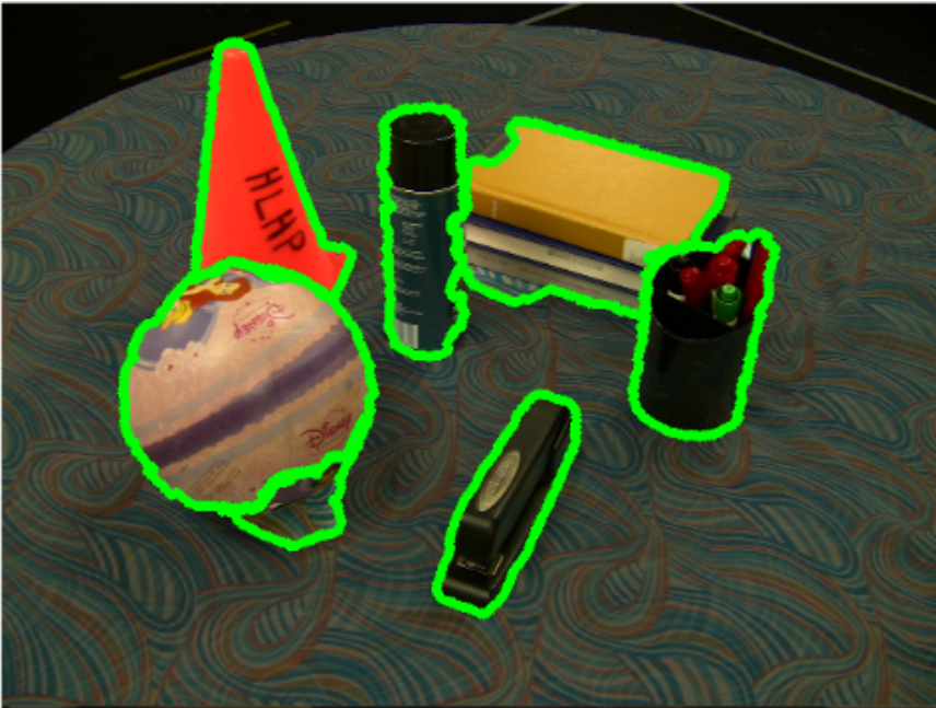
In fact, we’ve already seen an example of simple foreground/background segmentation: the GMM-based orange ball detector from project 1! But the approach we used there (train a GMM to recognize a range of colors characteristic of a specific object) had obvious limitations: it could only segment that one specific object, and needed a set of training data to do so. What if we want something more powerful and generalizable?

Motivation: Segmentation with Fixations

While there are many ways to approach segmentation, we’ll focus on a specific method proposed by Mishra, Aloimonos (our very own!), and Fah in their paper “Active Segmentation with Fixation”.

Note: our implementation differs slightly from that proposed by Mishra et al. Specifically, we replace the log-polar transform with a distance-based weighting, and add texture features. (More on this later.)

Most segmentation methods are “global”: they take in an entire image, and segment everything at once. But this differs fundamentally from what humans (and primates in general) do. When presented with a new scene, our eyes dart between many different points, spending more time on the things we perceive as more “interesting”. In the technical parlance, we say that our gaze “fixates” on the “salient” (most interesting/informative) points in the scene.

Our segmentation approach, “fixation-based segmentation”, takes inspiration from this phenomenon. Given an image and one or more “fixation points” identifying objects of interest, it segments the objects from the background.

Left: image with two fixation points (indicated by the green and red x’s). Right: the result of segmentation given those fixation points. (Source: Mishra et al.)

Graph-based Segmentation: a Toy Example

Before we get into the details of our fixation-based approach, let’s consider a basic example of graph-based binary segmentation (“binary segmentation” = segmentation into foreground and background).

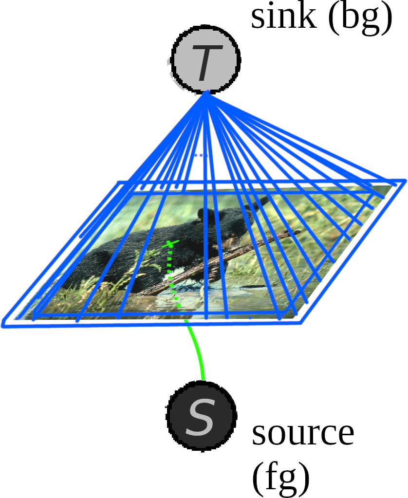
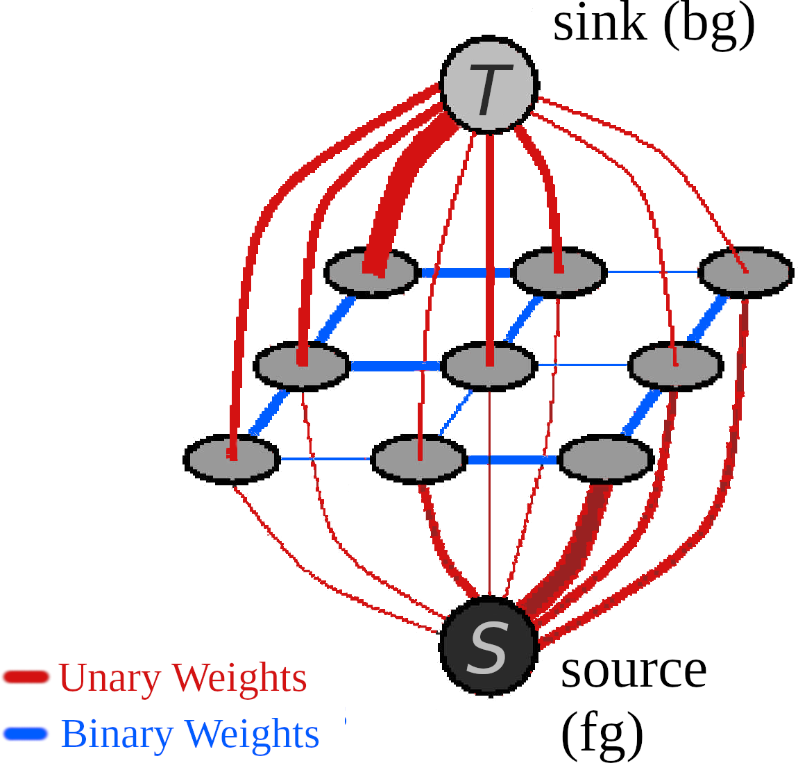
In the broadest sense, graph-based segmentation represents an image as a graph G = (V, E): the vertices V are regions of the image, connected by edges E which are weighted based on some measure of pixel similarity. The source vertex s is connected to some pixels which are known to be in the background, and the sink t is connected to pixels known to be in the foreground (these pixels are identified beforehand). To segment the image, we find a minimum-energy cut in that graph.

Consider the example shown below. For the sake of simplicity, the vertices are individual pixels, each of which is connected to its four adjacent neighbors. An edge is weighted simply based on the difference in intensity of the pixels it connects:

Min-cut segmentation of a simple 3x3 image. Nodes are pixels. In this illustration the thickness of an edge represents its weight. *Modified (with permission) from: Boykov, Yuri, and Gareth Funka-Lea. "Graph cuts and efficient ND image segmentation." International journal of computer vision 70.2 (2006): 109-131.*

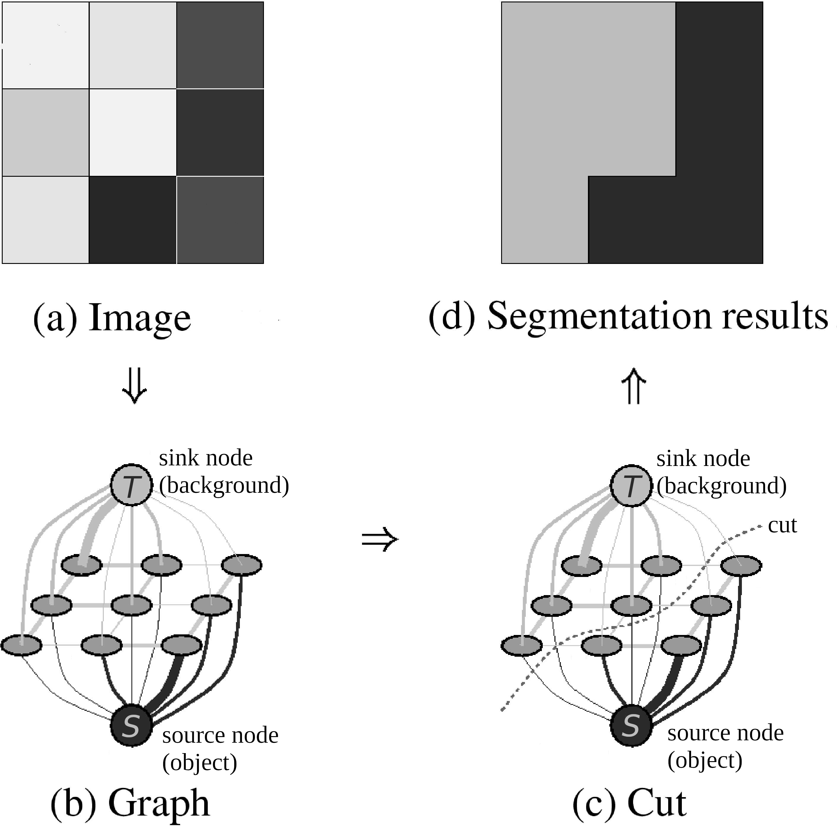
(While this setup is adequate for the purposes of this project, it doesn’t begin to cover the full complexity and diversity of graph-cut segmentation methods! If you’d like to learn more, we recommend these slides from Stanford as a starting point.)

Fixation-based Segmentation

Let’s see how we can extend this framework for fixation-based segmentation.

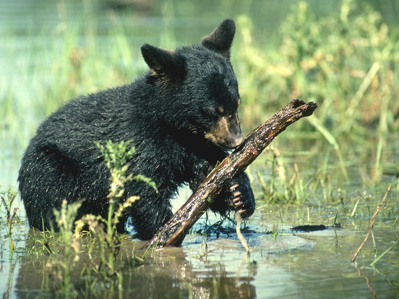
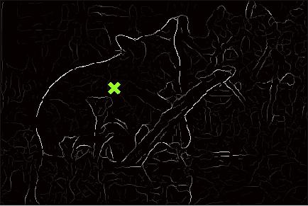
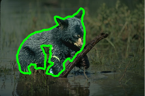
In fixation-based segmentation, we are given an image I and a “fixation” point $p_{fix}$ to identify the foreground object. As an example, let’s use this image:

*A typical grad TA at UMD. The green x marks the fixation point, p\_{fix}. Source: Mishra et al.

We can incorporate the fixation point into our graph very easily: just consider the “fixation point” to be the source s! Assuming that the object is entirely within frame (i.e. its outline doesn’t intersect with the bounds of the image), we can designate all of the boundary pixels to be the sink t.

The source is connected to the fixation point, p\_{fix}, and the sink is connected to *all* the outermost points of the image.

What about the edge weights? Unfortunately the simple “change-in-intensity” metric from before is too simplistic for more complicated images. Instead, we’ll use a higher-level feature: edges, as given by an edge detection algorithm (such as gPb - we’ll use it as a black box for this project.) Specifically, we’ll use a probabilistic edge boundary map, $I_{E}$: for each pixel, the probability (range [0,1]) that it is at the boundary between two regions of the image.

Boundary edge map I_E (found via gPb) for image I. (Source: Mishra et al.)

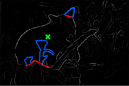
Unfortunately, there’s one more problem we have to address: as currently constructed, the algorithm inherently prefers shorter contours. To illustrate why (and why this is a problem), let’s use another example. In the figure below, we want to find the optimal contour in the disc for the red fixation point. In this case, the outer (white) circle is the actual boundary, while the inner (gray) circle is an internal boundary (analogous to the internal boundary created by the bear’s muzzle in the boundary edge map). Which contour will be the min-cut?

Fig 2 from Mishra et al.: (a) an example image. (b) The gradient edge map. (c) and (d) are the polar edge maps, generated by transforming the gradient edge map of the disc w.r.t the red and green fixations (respectively).

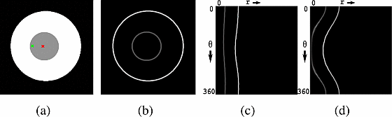
Well, in the edge map (b), the pixels of the outer ring have value 0.78, and the inner ring 0.39. The outer ring has radius 400, and the inner 100. So, the cost of the outer contour will be 61=(100×(1−0.39)), and internal contour 88=(400×(1−0.78)); thus the algorithm (incorrectly) chooses the inner contour.

To address this, we need to make the cost of a segmented region is independent of the area it encloses. One way to accomplish this is to transform the image into polar coordinates: “unrolling” the image in a circle around the fixation point. See (c) for an example of unrolling around the red fixation point. (Desirably, this transform also makes the optimal contour stable when the location of the fixation point within the object changes. See, for example, the green vs red fixation points in the fig below, with their corresponding polar transforms (c) and (d): the shape of the transformed contours change slightly, but this doesn’t change which one is optimal. Mishra et al. show that this property holds for general images in section 8.1 of their paper.)

• NOTE: for project 3, you shouldn’t actually transform the image into polar coordinates. The transformation introduces artifacts as theta approaches 0 and the pixels become more and more stretched. A better solution is to add an additional weighting term which is inversely proportional to the distance from the fixation point.

Alright, now that we’ve fixed the “shortcutting” problem, let’s re-run the segmentation:

Segmentation, after accounting for “shortcutting” problem. (Source: Mishra et al.)

That’s definitely an improvement! But there are noticeable mistakes: the segmentation erroneously includes some foreground vegetation, and excludes the bear’s left ear. If we look at $I_{E}$, the reasons for these mistakes become clear: to exclude the foreground vegetation, the contour would have to run all the way around it, at significant cost.

$I_{E}$ annotated to illustrate segmentation errors (red) vs groundtruth path (blue). (Modified from Mishra et al.)

Adding Additional Image Features

To eliminate these sorts of errors, we’ll have to go beyond the edge map, and incorporate other image features. For example, if our segmentation incuded color information, the green foreground vegetation would stand out starkly against the bear’s black fur.

We’ll add these new image features as an additional set of edge weights. We’ll call them unary weights, as they apply to an individual pixel (based on its color, texture, flow, etc.). Our original weights (based on $I_{E}$) are binary weights, as they describe the relationship between two pixels (i.e., the probability that there is a foreground/background boundary between two pixels).

• A unary weight applies to an individual pixel, representing the likelihood that pixel is in the foreground or background.
• A binary weight applies to an edge between two pixels, representing the likelihood that there is a foreground/background boundary between them.

Looking back to the initial example, unary weights are the connections between pixels and the source/sink node, and binary weights are the connections between pixels:

Unary and binary weights. (Modified from Boykov et al. Used with permission.)

Formal Problem Statement

Now, let’s define our problem formally. Set $P$ contains a node $p$ for each pixel in the image. We want to find a binary labeling for all the nodes, $f:p \mapsto l$, where $l_{p} = 0$ if $p$ is in the foreground, and $l_{p} = 1$ if $p$ is in the background. This labeling must minimize the energy function $Q(f)$:

• $U_{p}(l_{p})$ is the unary weight for $p$.
  • (If using more than one feature type (for example, color, texture, and flow), this is a weighted average of the different features: $aU^{color}(p) + bU^{text.}(p) + cU^{flow}(p)$ for $a+b+c = 1$.)
• $\Omega$ is the set of all pairs of adjacent nodes.
• $V(p,q)$ is the binary weight for the edge connecting points $p$ and $q$ :

• $\delta(l_{p},l_{q})$ indicates whether the edge is a fg/bg boundary:

• $I_{E}(p,q)$ is the boundary probability of the edge between $p$ and $q$. (i.e. $(I_{E}(p)+I_{E}(q))/2$.)
• Constants: (You might need to tune these!)
  • $\eta$ (=5): Gain for non-zero values in binary edge map.
  • $k$ (= 20): Default value for binary edge map (i.e. replaces zeros in $I_{pq}$)
  • $D$ (= 1e100): Source/Sink weight.
  • $\lambda$ (= 1000): Gain for binary weights.

Generating the Unary Weights

To determine our unary weights, we’ll use a familiar tool: the Gaussian Mixture Model! Specifically, we’ll train two separate GMM’s: one to classify foreground pixels ($G_{fg}$) and another to classify background pixels ($G_{bg}$).

• To train these GMMs, we’ll use the initial segmentation mask found with the binary weights: train $G_{fg}$ with all the pixels in the foreground region, and $G_{bg}$ with the pixels in the background. (Even thought the initial segmentation may be noisy, it’s usually not too noisy to use for training the GMMs.)

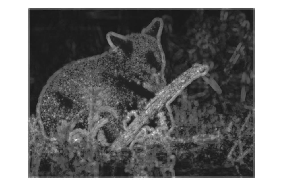
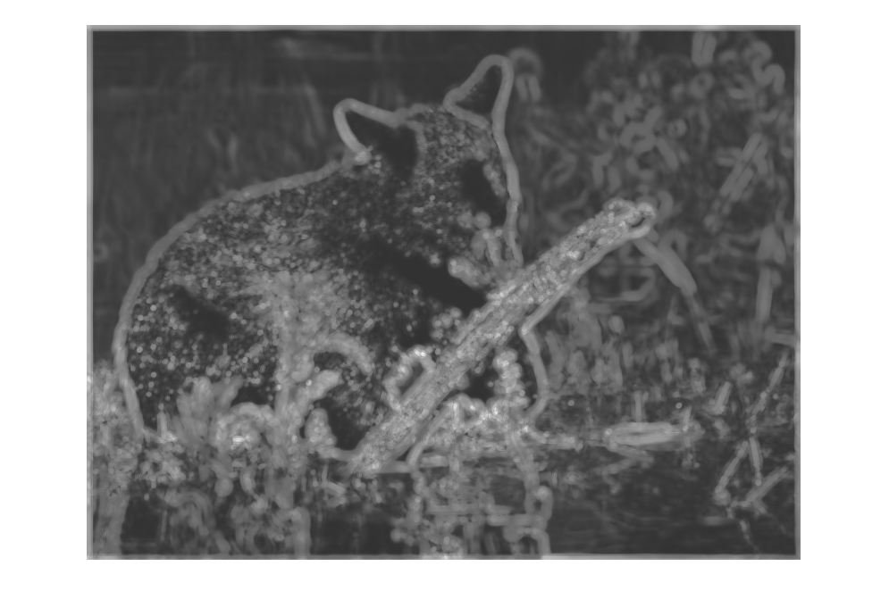
Once we’ve trained the GMMs, we use them to predict a probability that each pixel is in the foreground, and background. To start, let’s try using color. The following two maps show the log-likelihood of each pixel being in the foreground (as classified by $G_{fg}$) and background ($G_{bg}$):

Left: Background probability. Right: Foreground probability.

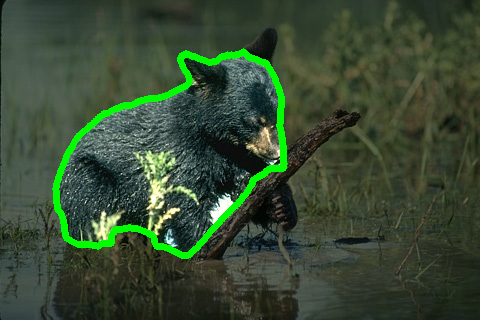
After adding these as unary weights to the graph and resegmenting, we get the following results:

Results of the second segmentation, with unary weights based on color features.

Much better!

Recap

Let’s take a moment to summarize the steps of our algorithm:

• Input: image $I$ and boundary edge map $I_{E}$.
  1. First segmentation – binary weights only (derived from $I_{E}$).
  • Output: segmentation labels $l_{initial}$ (1 (background) or 0 (foreground) for each pixel).

1. Compute unary weights:
   1. (If using texture/flow, generate texture/flow maps.)
   2. Train GMMs using color features: ${G^{color}_{fg}, G^{color}_{bg}}$
      • Training data for each is selected using the labels in $l_{initial}$.
      • If using texture/flow, do the same for ${G^{text.}_{fg}, G^{text.}_{bg}}$, etc.
2. Unary weights:
   • For point $p$, unary weight $U^{color}(p)$ = $[-log(p(p \vert G_{fg})) , -log(p(p \vert G_{bg})) ]$
   • *If using texture/flow as well, take a weighted average of the different features: $aU^{color}(p) + bU^{text.}(p) + cU^{flow}(p)$ for $a+b+c = 1$.

• Result: segmentation labels $l_{p}$ (1 (background) or 0 (foreground) for each pixel) for the image.

Appendix: Texture and Flow Features

Color-based segmentation worked well in our example image, but in other cases we may find other cues useful as well.

Texture:

An image texture is a set of metrics calculated in image processing designed to quantify the perceived texture of an image. Image texture gives us information about the spatial arrangement of color or intensities in an image or selected region of an image. (source: wikipedia)

For this project, we will use a simple metric, derived by convolving an image with a filter bank (i.e. a set of different filters). Filtering is at the heart of building the low level features we are interested in. We will use filtering both to measure texture properties and to aggregate regional texture and brightness distributions. A simple but effective filter bank is a collection of oriented Derivative of Gaussian filters. These filters can be created by convolving a simple Sobel filter and a Gaussian kernel and then rotating the result. Suppose we want o orientations (from 0 to 360◦) and s scales, we should end up with a total of s × o filters. A sample filter bank of size 2×16 is shown below:

Example of a filter bank of oriented derivative-of-gaussians.

Flow:

For sequences, we can improve segmentation further by including optical flow information. If the foreground and background have different relative motion, the optical flow may help us distinguish them. The optical flow map can be used to train a GMM, in the same way as was done for color and texture. (For more information on optical flow, see the lecture slides.)