This article is written by Nitin J. Sanket.

Table of Contents:

• Introduction to perception in an intelligent system
• Sample Vision Pipeline
• Color Imaging
• RGB and other Color Spaces
• Color Classification
  • Color Thresholding
  • Color Classification using a Single Gaussian
  • Color Classification using a Gaussian Mixture Model (GMM)
  • Different cases for $\Sigma$ in GMM
• Estimation of distance to the orange ball

Introduction

In this lecture, we’ll introduce how a camera forms an image, and how we can identify objects of a known color by manipulating color-spaces.

But first, a bit of motivation. An intelligent system senses the world and responds in some way. For a robot, this means interacting with the environment via its actuators:

Intelligent Agent (Robot) interacting with the environment and sensing the world.

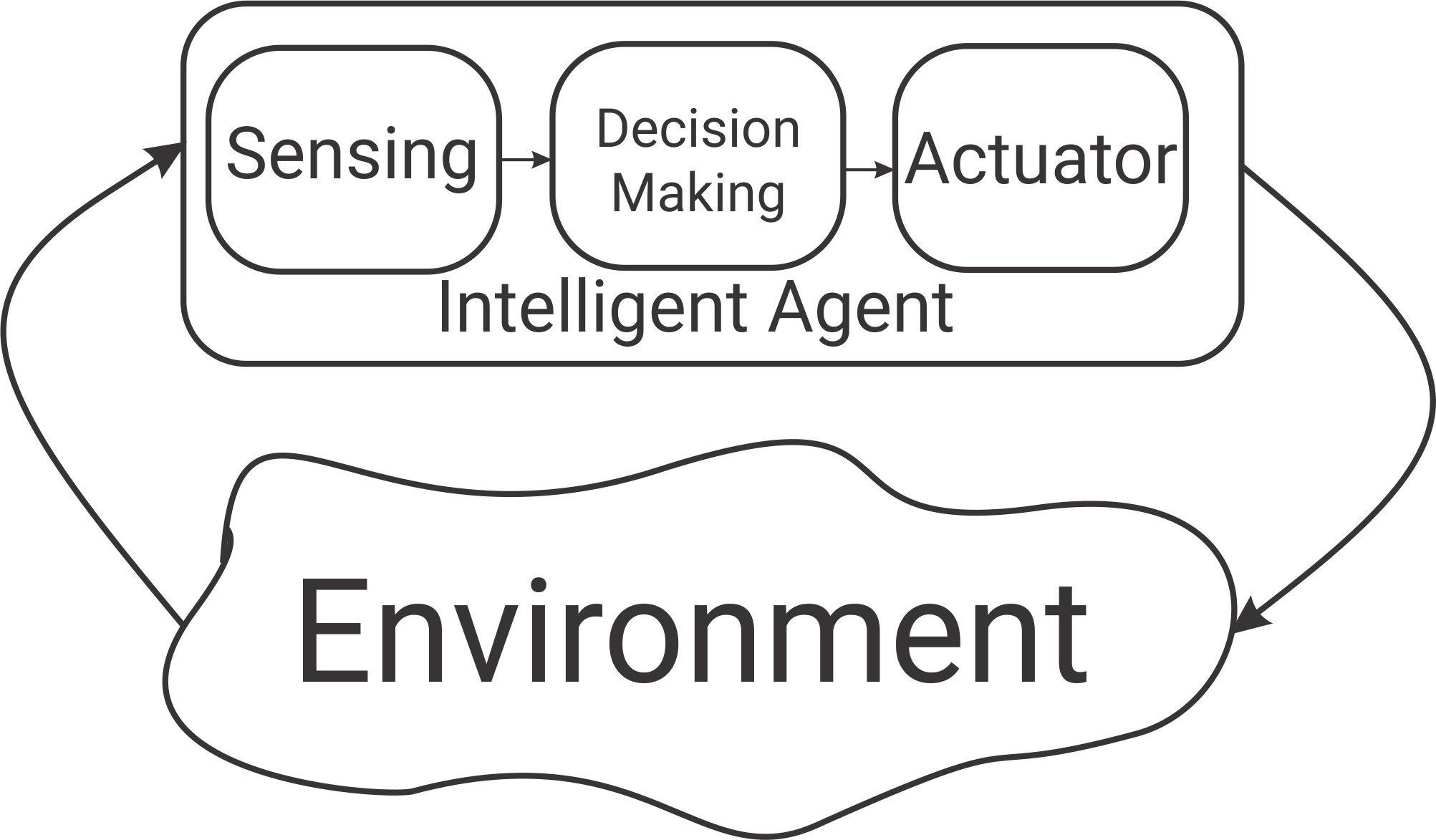
The robot’s sensors and movements are noisy. For example, an autonomous car might know that it is about 5ft. away from a pedestrian, give or take a few inches. The robot can improve its estimate by combining information from multiple sensors. A good estimate of the world also helps the robot interact with its environment more accurately: whenever a robot moves, because its motors are not perfect, its movements are noisy. To counteract this, the robot can continuously monitor the state of the world to make sure it has accomplished what it intended to.

A sample Vision Pipeline in an intelligent agent

As an introduction to robotic visual perception, you’ll be implementing a simplified vision system for a soccer playing robot.
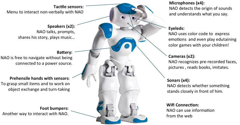
Meet Nao, a 58cm high humanoid robot which can walk, pick-up things, and even talk. Its sensors include two cameras (one front and one facing down at an angle), some sonar distance sensors, and contact sensors (essentially just buttons). Its onboard CPU is an Intel Atom. Notably, Nao is used in the Robocup Standard Platform League, where two teams of five robots square off in a soccer match. The teams are completely autonomous, and all computation must be done on the robots themselves. To succeed, the robots’ algorithms must be robust, fast, and lightweight.
In project 1, you’ll get a flavor of what goes behind the scenes in a typical vision system for a Robocup player. Your objective is to detect the soccer ball and estimate the distance to it. Doesn’t it sound cool?

Nao robot.

In Robocup, the soccer field is bright green, the ball is bright orange, and the goal-posts are bright yellow. If we separate the image into these three color classes, we can identify if/where these objects are in the image. A sample pipeline is: 1) the robot acquires an image, 2) classifies each pixel as belonging to one of the color classes (“soccer-field-green”, “ball-orange”, or “goal-post-yellow”), and 3) groups the labled pixels and classifies the objects. This information is then passed on to a higher-level planning algorithm, which makes high-level decisions like “kick the ball”.

Color Imaging

To build our vision pipeline, we need to understand how digital images are formed. A simple black-and-white/grayscale sensor works by measuring the number of photons per second hitting each pixel. Think of a grayscale image as a 2D array of pixels where each pixel is one element of the array. The values of the array correspond to the amount of light (number of photons) that hit each pixel in some amount of time (generally the shutter speed of the camera). If you open the PRO mode on your phone’s camera (or have a fancy DSLR) you’ll see the four most important factors in image formation: focal length, aperture, ISO, and shutter speed. A combination of the last three controls the average brightness of the image (and is called the “exposure triangle” in photography lingo).

The focal Length tells you how wide the field of view (FOV) of the lens is. The smaller the focal length, the more angle you see and vice-versa. For example, an 8mm lens can have an FOV of 110$^\circ$ and a 50mm lens can have an FOV of 32$^\circ$.

The aperture is the amount of opening of the lens. For example, the lens can have a diameter of 70mm but only 5mm might be collecting light. Why use only 5mm of a 70mm diameter lens? The answer lies in the depth of field. The depth of field controls how the range of distances from the camera in which an object appears in focus. A wide opening in the lens lets in a lot of light but has a shallower depth of field; thus, which means that only a small range of distances will appear in focus. A shallow depth of field can be used for artistic effect, for example shooting a portrait where the subject is in focus and the background blurry. A large depth of field – a small aperture – is more desirable for robotic perception, as we want to capture as much detail in the scene as possible. However, aperture size is a trade-off: a smaller aperture also means less light is let into the lens, reducing performance at night or low-light. There is no silver bullet to solve this problem. But a rule of thumb in vision/robotics is to disregard focus very close to the camera (say, within 1m), and set the aperture large enough to let in enough light, but small enough that objects further than 1m are in focus. (Note, a very small aperture also leads to an effect called “diffraction” which leads to a “softer” image.)

The next factor controlling the brightness of the image is the ISO. To understand it, you’ll need to understand some of the electronics behind a digital image sensor. Each pixel is generally a capacitor/transistor which converts photos/light into some voltage, which can be measured by a circuit in the camera. Think of this as light turning a dial/volume knob, telling you how much light hits a particular pixel. The volatge level measured per pixel can be amplifed by a number, much as you can amplifying the volume on your headphones. ISO controls this amplification factor. As you might expect, a higher ISO means a brighter image and vice-versa. Why not just set a small aperture and increase your ISO to the maximum value? Increasing ISO comes at a cost: a lot of noise. So, one must find a balance between amplification and noise.

Effects of ISO, Aperture, Shutter speed on the image.

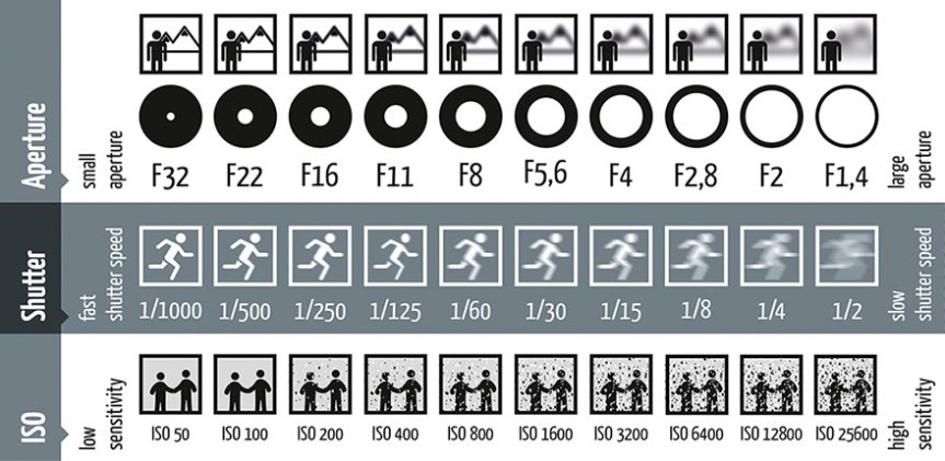
The last factor in the exposure triangle is the shutter speed. This is the amount of time the camera/imager collects light. The voltage measured will be a sum of all the photons collected while the shutter is active/open. A longer shutter speed lets in more light, but will blur any motion.

The camera’s auto mode generally selects the best balance of all the exposure triangle parameters based on some heuristic. (Look at this cool paper which cheats the exposure traingle with Deep Learning. This paper can predict the noiseless detail which would be obtained from a long exposure given a super short noisy exposure. What a time to be alive! A version of this is used in the Google Pixel phones for the night mode.)

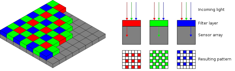
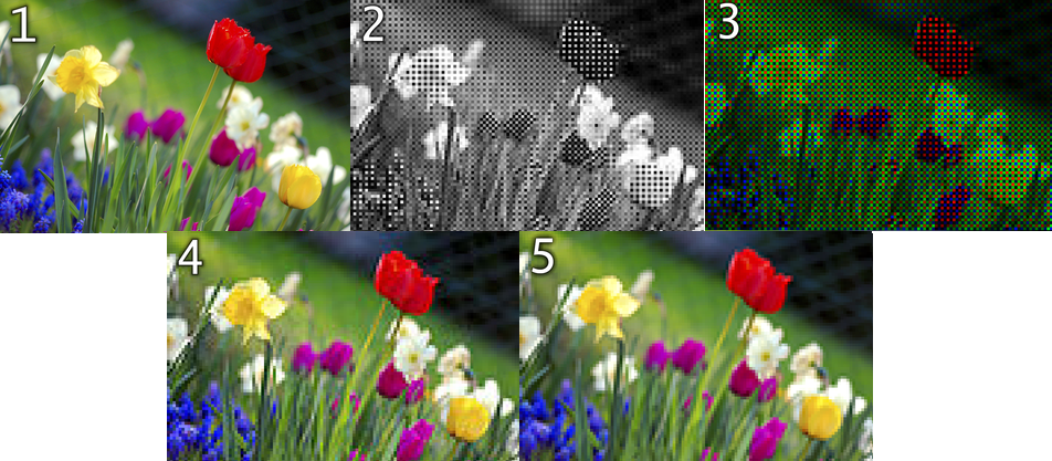
To sense color, rather than grayscale, the image sensor must be able to differentiate between different wavelengths of light. A simple way of doing this is to split each pixel into three “sub-pixels” of red, green, and blue. One can select a color by using the dye of the same color on the sub-pixel (grayscale has a transparent dye). But having three sub-pixels for each pixel is very expensive, and is generally only used in high end cameras costing thousands of dollars. More commonly, the sub-pixels are tiled in a pattern caled the “Bayer pattern”, shown below. The missing colors are interpolated using a simple interpolation algorithm. The RGB image is represented as a three dimentional array (width x height x 3) on the computer.

Left: The Bayer arrangement of color filters on the pixel array of an image sensor. Right: Profile/cross-section of sensor. </a>

1. Original scene. 2. Output of a 120\(\times\)80-pixel sensor with a Bayer filter. 3. Output color-coded with Bayer filter colors. 4. Reconstructed image after interpolating missing color information. 5. Full RGB version at 120\(\times\)80-pixels for comparison (e.g. as a film scan might appear).

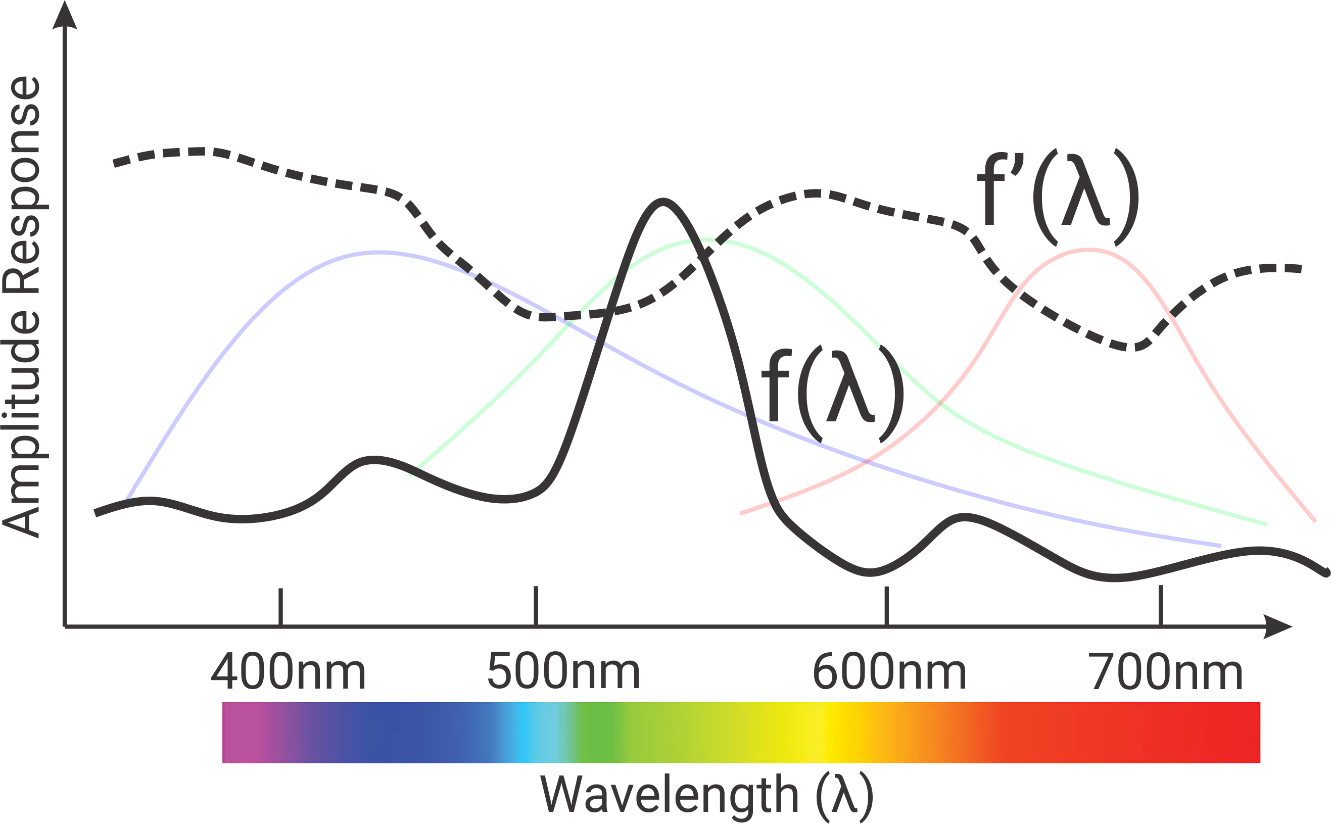
Why use RGB for the color image and not something else? The answer lies in the human retina, which has 3 types of cone cells: red, green, and blue. We can model the activation/response/sensitivity of a cone cell as some unimodal distribution function (a distriution with only one peak). The three kinds of cone cells are sensitive to Small ($S(\lambda)$), Medium ($M(\lambda)$) and Long ($L(\lambda)$) wavelengths of visible light which coincide with red, green and blue colored light. Think of these cone cells as very sensitive to red, green or blue light. Any scene reflects a arbitrary spectrum of light (or signal represnted as $f(\lambda)$). One might wonder what the response of red sensitive cone cells will look like on this input light spectrum. One can represent the response of the S, M and L detectors/cone cells by a super simplified model given by:

Note that a completely different scene can reflect a different spectrum of light ($f'(\lambda)$). Because of the way the detectors work, $S_{res}, M_{res}, L_{res}$ could have the exact same value. This means that one cannot distinguish the two scenes by color. This is because the eyes “see” a 3D projection of the $\infty$-dimensional hilbert space of the spectrum. This is mathematically represented as $\mathbb{R}^\infty \rightarrow \mathbb{R}^3$. Color blindess is the result of missing one of the receptors or the S, M, L receptors become too similar to each other. This in-turn reduces the dimentionality from three to two or one. This is in a sense taking the PCA of the infinite dimensional spectrum in your eyes.

The response of S, M and L detectors to \(f(\lambda)\) and \(f'(\lambda)\) might look exactly the same. This is because both \(f(\lambda)\) and \(f'(\lambda)\) are \(\infty\)-dimensional functions and only 3-dimensions of it are measured by the RGB (S, M and L) cone cells.

RGB and other Color Spaces

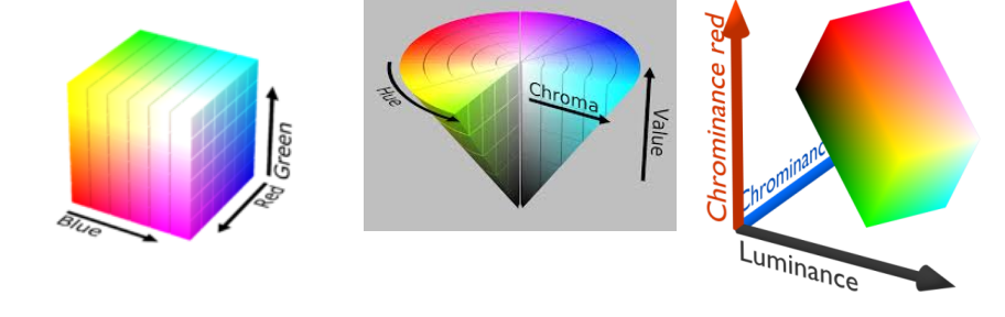
The colors RGB can be represented in a 3D vector space. Think of this as X, Y and Z co-ordinate of a vector space representing colors. In most generic cameras, 8-bits are used to represent each color channel (the values range from 0-255). This means that an RGB pixel has 24-bits of data represented as a triplet of [Red, Green, Blue]. A value of [0,0,0] represents pure black, [255,255,255] represents pure white, [255,0,0] represents pure red and so on. Gray is any color with equal values for all the three channels. We can visualize RGB space in three dimensions as a unit cube (for an 8-bit color space, we’d divide by 255 to make it unit length). But if colors are just a vector space, can’t we transform them to make a different space? Indeed, we can; this gives rise to color spaces like Hue Saturation Value (HSV) and Luminance and chroma (YCbCr). If $[R, G, B]$ represents a sample color in the RGB color space, then the equivalent HSV color space value is given by,

Hue is calculated as follows:

Saturation is calculated as follows:

Value is calulated as follows:

If RGB space was a pretty unit cube, then what do these weird transformation spaces look like? The unit RGB cube in HSV space looks like a cone (cool eh?). HSV is very popular and is used in NTSC, PAL, SECAM and other television broadcast systems.

If $[R, G, B]$ represents a sample color in the RGB color space, then the equivalent YCbCr color space value is given by,

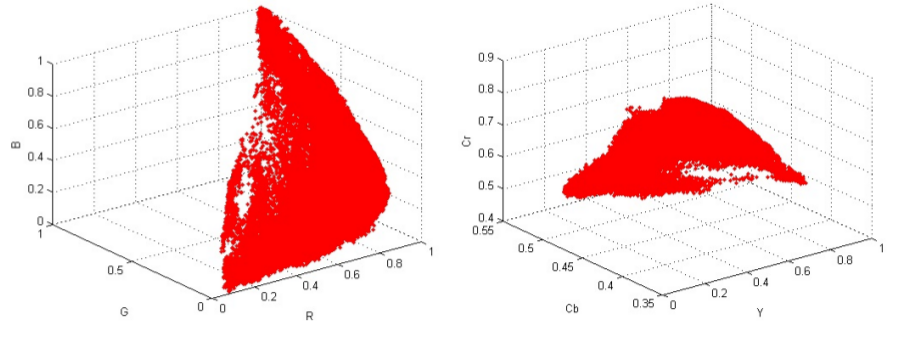
Keen readers might observe that HSV is a non-linear transformation of the RGB color space, and YCbCr is a linear transformation. The RGB color cube looks like a rotated cuboid in YCbCr space. (Look at rgb2hsv, hsv2rgb, rgb2ycbcr, ycbcr2rgb functions in MATLAB and play around. A fun exercise would be to try to plot the RGB color cube in different color spaces! )

Left to right: Represenation of RGB color cube in RGB, HSV and YCbCr color spaces.

Nao robot view in RGB, HSV and YCbCr colorspaces.

Color Classification

Back to project 1: the Nao robot wants to classify each pixel as a set of discrete colors (i.e., green of the grass field, orange of the soccer ball, and yellow of the goal post). Particularly, we are interested in finding the orange pixels because this represents the ball. As mentioned before, in RGB color space each pixel is represented as a vector in $\mathbb{R}^3$. Let us define the problem mathematically. Say each pixel is represented by $x=[r,g,b]^T \in \mathbb{R}^3$. There exist $l$ color classes. We want to model the probability of a pixel belonging to a color class $C_l$ given the pixel value $x$, denoted by $p(C_l \vert x)$.

Color Thresholding

If we assume each pixel belongs to only one color class, i.e., color classes are mutually exlusive [1], the hard classification problem can be mathematically defined as follows:

$C_l^*(x) = \underset{C_k}{\operatorname{argmax}} p(C_k\vert x)$

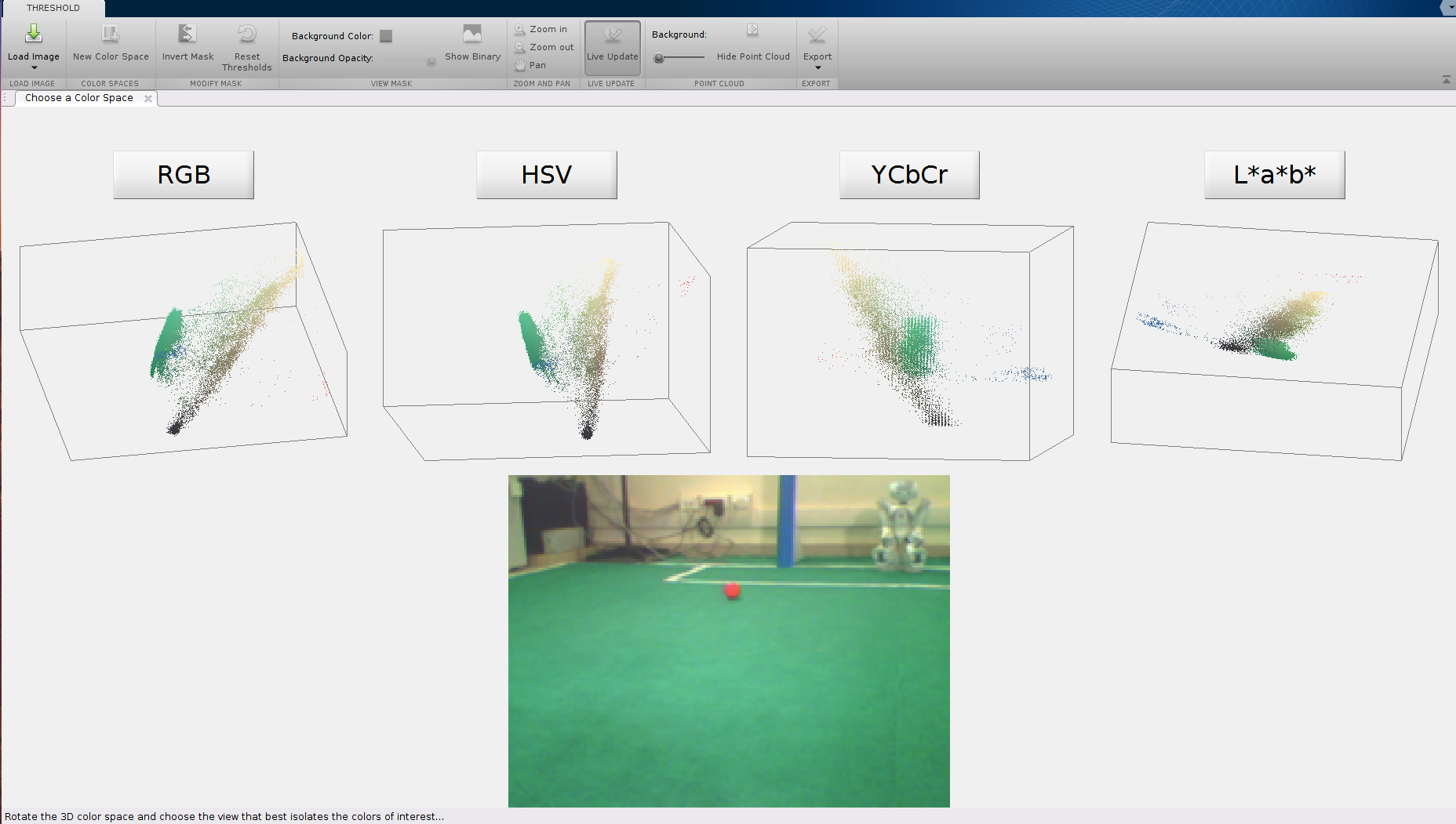
Here, $C_l^*(x)$ represents the most probable color class that pixel belongs to. For eg. if the color is closer to orange than red then the pixel will be called orange. This can be done using the Color Thresholder app in MATLAB. In RGB space, thresholding can be thought of selecting pixels in a cube defined by some minimum and maximum value in each channel (RGB), i.e., you are selecting all the pixels in a cube whose faces are defined by the minimum and maxmimum value in each channel. This can be mathematically formulated as:

where $x^r, x^g, x^b$ represent the red, green and blue channel values of a particular pixel.

Color Thresholder app in MATLAB with a sample input image from a nao's camera.

[1] This is like saying “if a pixel is classified as orange it cannot be classified as red” though in reality a red pixel could have some amount of orange and vice-versa. This comes from that fact that the camera sensor percieves a 3-dimensional projection of the $\infty$-dimensional hilbert space projection of the light spectrum.

Color Classification using a Single Gaussian

This is good for most basic cases but is bad for robotics because we said that everything (sensors and actuators) is noisy and we want to model the world in a probabilistic manner. This means that instead of saying a pixel is orange/red we want to say that the pixel is orange with 70% probability and red with 30% probability. This is denoted as $p(C_l\vert x)$ as mentioned before. Because we are in 2018 and everything is machine learning driven, let us treat the problem in hand as a machine learning problem. Let us say each pixel is being classified by a binary classifier per class (i.e., we have one classifier per color we want to classify). If we want to classify a pixel as red, orange or green we have a total of three classifiers one for each color. Let us formulate the problem mathematically. In each classifier, we want to find $p(C_l \vert x)$. Here $C_l$ denotes the color label, in our case they will be green or orange or yellow. So as you expect the green classifier will give you the following $p(Green \vert x)$, i.e., probability that the pixel is green. Note that $1 - p(Green \vert x)$ gives the probability that the pixel is not green which includes both orange and yellow pixels.

Estimating $p(C_l \vert x)$ directly is too difficult. Luckily, we have Bayes rule to rescue us! Bayes rule applied onto $p(C_l \vert x)$ gives us the following:

$p(C_l \vert x)$ is the conditional probability of a color label given the color observation and is called the Posterior. $p(x \vert C_l)$ is the conditional probability of color observation given the color label and is generally called the Likelihood. $p(C_l)$ is the probability of that color class occuring and is called the Prior. The prior is used to increase/decrease the probability of certain colors. For eg., one would generally see more green in the robocup because the field is green in color and the robot mostly looks at the ground. If nothing about the prior is known, a common choice is to use a uniform distribution, i.e., all the colors are equally likely. Let us consider the problem of color classification as a supervised learning problem now. Supervised means that we have some number of “training” examples from which we can understand the color we are looking for.

For the purpose of easy discussion, let us say we want to classify a pixel as orange. To do this we need to make the computer know how orange color looks like. Say we have a number of training samples of the color orange. You might ask why do we need so many samples? The answer is lighting and sensor noise changes the way orange looks in the image every so slightly and the computer has to learn all these different shades of orange. The next question one might ask, how many samples do we need? This is a hard question to answer. It depends on the variety more than quantity of samples. It is better to have samples with more variation you want to cater to than a lot of very similar looking samples of data. Let us mathematically model the right hand side of $p(Orange \vert x)$. As we discussed earlier, Prior can be modelled as a uniform distribution, i.e., $p(Orange)=0.5$ and $p(\sim Orange)=0.5$ (probability of not orange). The Likelihood is generally modelled as a normal/gaussian distribution given by the following equation:

Here, $\vert \Sigma \vert$ denotes the determinant of the matrix $\Sigma$. The dimensions of the above terms are as follows: $\Sigma \in \mathbb{R}^{3 \times 3}, x,\mu \in \mathbb{3 \times 1}, p(x \vert Orange) \in \mathbb{R}^1$.

You might be asking why we used a Gaussian distribution to model the likelihood. The answer is simple, when you average a lot of (theoretically $\infty$) independently identically distributed random samples, their distribution tends to become a gaussian. This is formally called the Central Limit Theorem.

All the math explanation is cool but how do we implement this? It’s simpler than you think. All you have to do is find the mean ($\mu$) and covariance ($\Sigma$) of the likelihood gaussian distribution. Let us assume that we have $N$ samples for the class ‘Orange’ where each sample is of size $\mathbb{R}^{3 \times 1}$ representing the red, green and blue channel information at a particular pixel. The empirical mean $\mu$ is computed as follows:

here $i$ denotes the sample number. The empirical co-variance $\Sigma$ is compted as follows:

Clearly, $\mu \in \mathbb{3 \times 1}$ and $\Sigma \in \mathbb{R}^{3 \times 3}$. $\Sigma$ is an awesome matrix and has some cool properties. Let us discuss a few of them.

The co-variance matrix $\Sigma$ is a square matrix of size $d \times d$ where $d$ is the length of the vector $x$, i.e., $\Sigma \in \mathbb{R}^{d \times d}$ if $x \in \mathbb{R}^{d \times 1}$. For the RGB case, $d=3$. $\Sigma$’s diagonal terms denote the variance and the off-diagonal terms denote the correlation. Let us take the example of the RGB case. If $x = [R, G, B]^T$, then

Observe that the above matrix is a square matrix and is a symmetric matrix. Here, $\sigma_R, \sigma_G, \sigma_B$ denote the variance in each of the individual channels. $\sigma_R^2, \sigma_G^2, \sigma_B^2$ are the variance in each of the R, G and B channels. $\sigma_R \sigma_G, \sigma_G \sigma_B, \sigma_R \sigma_B$ are the correlation terms and show the co-occurence of one channel over other. Mathematically, it signifies the vector projection of one channel over the other.

An important property to know about $\Sigma$ is that it is a Positive Semi-Definite (PSD) Matrix and is denoted mathematically as $\Sigma \succeq 0$. This means that the eigenvalues are non-negative (either positive or zero). This physically means that you cannot have a negative semi-axes for the ellipse/elliposoid which makes sense. The eigenvectors of $\Sigma$ tell you the orientation of the elliposoid in 3D. A function like this can help you plot the covariance ellipsoids.

Now that we have both the prior and likelihood defined we can find the posterior easily:

Because we just want to find the colors by some thresholding later, we can drop the denominator in the above expression if we don’t care about the absolute scale of the probability summing to 1. For most thresholding purposes, we can do the following approximation:

So using the following expression one can identify pixels which are ‘Orange’ (or confidently Orange).

Here, $\tau$ is a user chosen threshold which signifies the confidence score. This method definitely works much better than the simpler color thresholding method. All your data is being thresholded by an ellipsoid (3D ellipse) instead of a cube as before. You might be wondering why a gaussian looks like an ellipsoid? The covariance matrix represents the semi-axes of the ellipsoid. In fact the inverse of square root of diagonal values of $\Sigma$ gives the semi-axes of the ellipsoid. As you would expect if $x \in \mathbb{R}^{2 \times 1}$, the gaussian would look like an ellipse. Learn more about these cool gaussians here.

Modelling the likelihood as a gaussian is beneficial because a little light variation generally makes the colors spread out in an ellipsoid form, i.e., the actual color is in the middle and color deviates from the center in all directions resembling an ellipse. This is one of the major reasons why a simple gaussian model works so well for color segmentation.

Color Classification using a Gaussian Mixture Model (GMM)

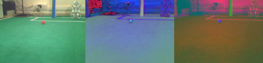
However, if you are trying to find a color in different lighting conditions a simple gaussian model will not suffice because the colors may not be bounded well by an ellipsoid.

Datapoints for the ball plotted in RGB and YCbCr colorspaces. Observe how the enclosing shape is of a weird shape. It would be ideal to create a custom color-space which converts this weird shape into some simple shape which can be enclosed like a cube or a cuboid or a sphere or an ellipsoid. Designing a space like that is generally not trivial hence we emply a method of fitting this weird shape as a sum of simple shapes like an ellipsoid.

In this case, one has to come up with a weird looking fancy function to bound the color which is generally mathematically very difficult and computationally very expensive. An easy trick mathematicians like to do in such cases (which is generally a very good approximation with less compuational cost) is to represent the fancy function as a sum of known simple functions. We love gaussians so let us use a sum of gaussians to model our fancy function. Let us write our formulation down mathematically. Let the posterior be defined by a sum of $K$ scaled gaussians given by:

Here, $\pi_i$, $\mu_i$ and $\Sigma_i$ respectively define the scaling factor, mean and co-variance of the $k$^th gaussian. The optimization problem in hand is to maximize the probability that the above model is correct, i.e., to find the parameters $\pi_k, \mu_k, \Sigma_k$ such that one would maximize the corectness of $p(C_l \vert x)$. Just a simple probability function doesnt have very pretty mathematical properties. So a general trick mathematicians/machine learning people follow is to take the logarithm of the probability function and maximize that. This works well because of the monotonicity of the logarithm function. This setup is formally called Maximum Likelihood Estimation (MLE) and can be mathematically written as:

where $N$ is the number of training samples. The above is not a simple function and generally has no closed form solution. To solve for the parameters $\Theta = \{ \mu_1, \mu_2, \cdots, \mu_k, \Sigma_1, \Sigma_2, \cdots, \Sigma_k, \pi_1, \pi_2, \cdots, \pi_k\}$ of the above problem, we have to use an iterative procedure.

• Initialization: Randomly choose $\pi_i, \mu_i, \Sigma_i \qquad \forall i \in [1, k]$
• Alternate until convergence:
  • Expectation Step or E-step: Evaluate the model/Assign points to clusters Cluster Weight $\alpha_{i,j} = \frac{\pi_i p(x_j \vert C_i)}{\sum_{i=1}^k \pi_i p(x_j \vert C_i)}$ \(j\) is the data point index, \(i\) is the cluster index.
  • Maximization Step or M-step: Evaluate best parameters $\Theta$ to best fit the points
  $$\mu_i = \frac{\sum_{j=1}^N \alpha_{i,j} x_j}{\sum_{j=1}^N \alpha_{i,j}}$$ $$\Sigma_k = \frac{\sum_{j=1}^N \alpha_{i,j} (x_j-\mu_i)(x_j-\mu_i)^T}{\sum_{j=1}^N \alpha_{i,j}}$$ $$\pi_i = \frac{1}{N}\sum_j \alpha_{i,j}$$

Convergence is defined as $\sum_i\vert \vert \mu_i^{t+1} - \mu_i^{t}\vert \vert \le \tau$ where $i$ denotes the cluster number, $t$ denotes the iteration number and $\tau$ is some user defiened threshold. To understand more about the mathematical derivation which is fairly involved go to this link.

Now that we have estimated/learnt all the parameters in our model, i.e., $\Theta = \{ \mu_1, \mu_2, \cdots, \mu_k, \Sigma_1, \Sigma_2, \cdots, \Sigma_k, \pi_1, \pi_2, \cdots, \pi_k\}$ we can estimate the posterior probability using the following equation:

Finally, one can use the following expression to identify pixels which are ‘Orange’ (or confidently Orange).

here $\tau$ is some user defined threshold.

Different cases for $\Sigma$ in GMM

We said that we were modelling our fancy functions as a sum of simple functions like a gaussian. One might wonder why cant we make further asumptions about the gaussian. Yes we can! The gaussian we described before uses an ellipsoid, i.e., all the diagonal elements of $\Sigma$ are different. One can say that all our diagonal elements are the same and non-diagonal elements are zero, i.e., $\Sigma$ has the following form:

here $\sigma$ is a parameter to be estimated. You might be wondering what shape a $\Sigma$ like the one described above represents. It’s simple, a sphere! This gives lesser flexibility in fitting the model as the shape is simpler but has lesser number of parameters. A comparison of GMM fit on the data using spherical $\Sigma$ and elliposoidal $\Sigma$ is shown below:

Left: Datapoints of the orange ball and GMM fit using spherical \(\Sigma\). Right: GMM fit using ellipsoidal \(\Sigma\). Notice that the ellipsoidal variant has less non-orange pixels which will be classified as orange, i.e., lesser false positives and false negatives and is more accurate.

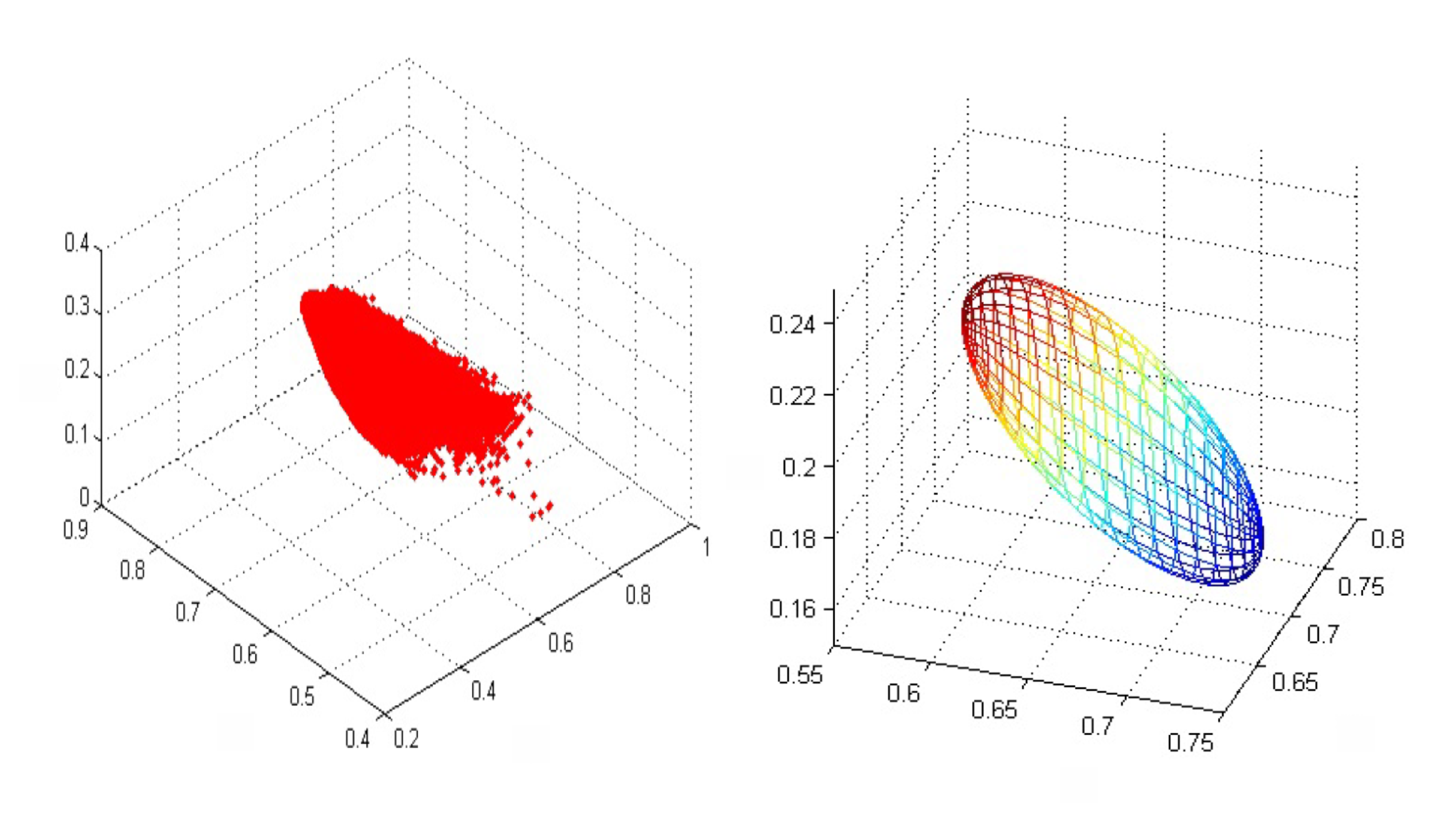
One might think, what if I design a custom transformation to create a new colorspace from RGB where the data points are enclosed in a simple shape like an ellipsoid? That would work wonderfully well. I designed a custom colorspace to do exactly that (which is my secret recipe). You will have to figure out your own secret recipe to do it. The datapoints and the GMM fit for this colorspace is shown below:

Left: Datapoints of the orange ball in the custom colorspace. Look at how the datapoint space looks like an ellipsoid Right: GMM fit using ellipsoidal \(\Sigma\). Notice that the GMM fit looks exactly like one single gaussian which shows that the performance of GMM over this colorspace would exactly be the same as a single gaussian fit. This is very beneficial because we can reduce the computation cost of training and testing significantly.

Estimation of distance to the orange ball

Nao robot looking at the ball from it's bottom camera.

Orange ball candidates after thresholding using GMM. One can remove the noise using morphological operations.

Orange ball looks different from different distances (\(d\)) and different head tilt angles (\(\theta\)). See how the ellipse's shape and size changes with repsect to distance and angle. It is not very easy to separate the effects of distance and angle on the shape and size of the ball on the image.

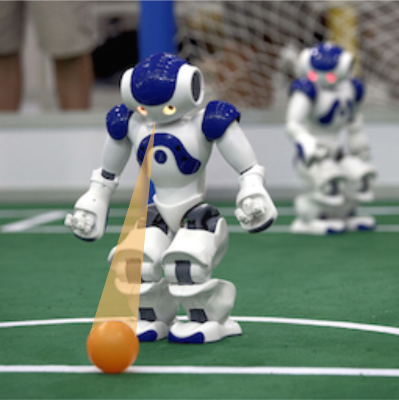
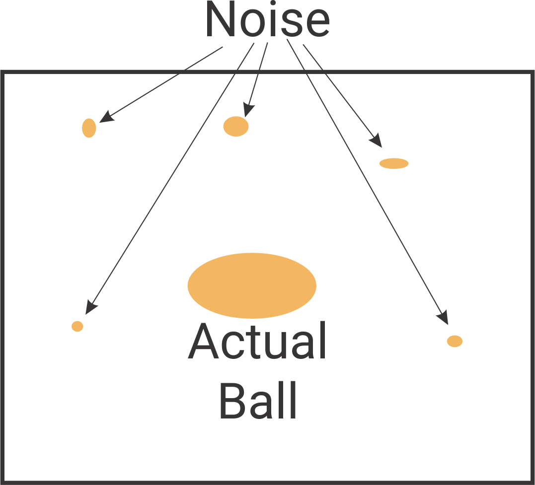
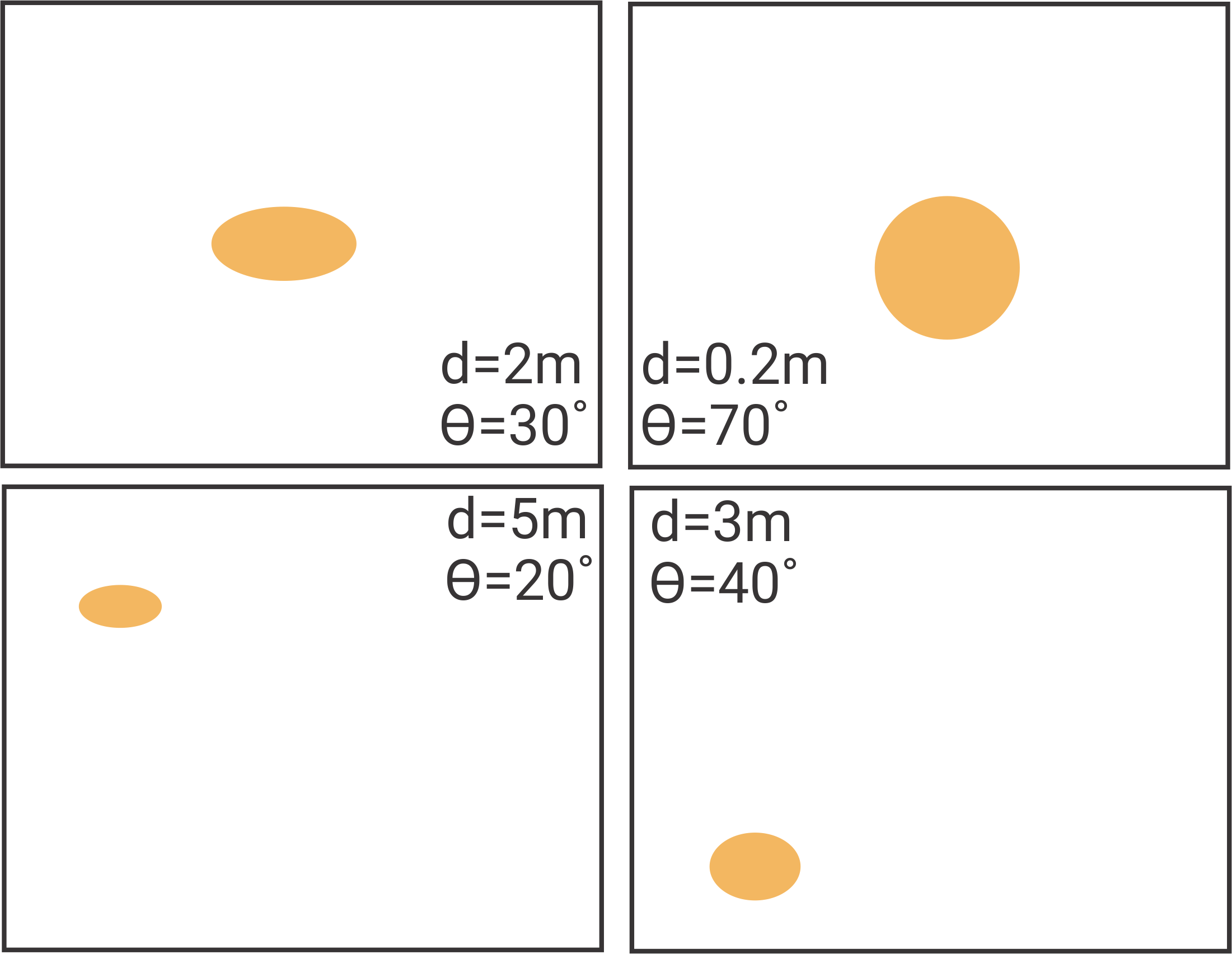
Now that we have robustly estimated the pixels which are ‘Orange’, we want to identify the pixels which belong to the orange ball and eventually find the distance to the ball. First step, let us identify the pixels which belong to the orange ball. This is relatively easy, one can use simple morphological operations available in MATLAB to do it. Look at bwmorph, regionprops functions in MATLAB. For the second step, one could just fit a simple parametric model (choose a model of your choice) to estimate distance from different parameters based on the image. For eg. area of the ball on the image decreases with distance (generally follows a inverse square curve). Use the data provided and any freature you like (regionprops from MATLAB is very handy) and the MATLAB function fit to obtain a model to estimate distance. For a more fancy method look at this paper.

Congrats! You have now built a robust vision system to identify an orange ball, estimate distance to it on a nao robot for robocup soccer.