Image Classification Using Convolutional Neural Networks
Table of Contents:
Deadline
11:59 PM, May 17, 2019
Introduction
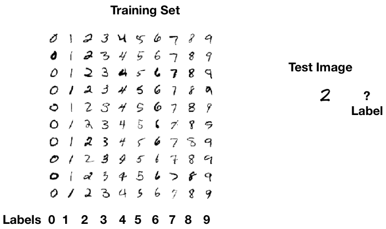
In this project you will implement a convolutional neural network (CNN). You will be building a supervised classifier to classify MNIST digits dataset.
Supervised classification is a computer vision task of categorizing unlabeled images to different categories or classes. This follows the training using labeled images of the same categories. You will be provided with a data set of images of MNIST digits. All of these images will be specifically labeled as a specific digit. You would use these labeled images as training data set to train a convolutional neural network. Once the CNN is trained you would test an unlabeled image and classify it as one of the ten digits. This task can be visualized in Figure 1.
Architecture
Your training and test step would contain the pipeline shown in Figure 2
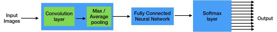
You are provided a framework for a single convolution layer (convolution + subsampling), a fully connected neural network with Sigmoid activation function, and a cross-entropy softmax layer with ten outputs. Next few sections present a description of each of these components of this network.
Fully Connected Layer
In a fully connected layer each neuron is connected to every neuron of the previous layer as shown in Figure 3
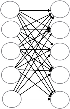
Each of these arrows (inputs) between the layers is associated with a weight. All these input weights can be represent by a 2-dimensional weight matrix, W. If the number of neurons in this layer is nc and the number of neurons in the previous layer is np, then the dimensionality of the weight matrix W will be nc x np. There is also a bias associated with each layer. For the current layer we will represent it by a vector, b, with a size of nc x 1. Therefore, for a given input, X, the output, Z, of a fully connected layer is given by the equation:
Z = WX + b
Convolutional layer
We will begin with a brief description of cross-correlation and convolution which are fundamental to a convolutional layer. Cross-correlation is a similarity measure between two signals when one has a time lag, represented in the continuous domain as
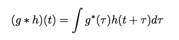
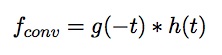
Convolution is similar, although one signal is reversed
They have two key features, shift invariance and linearity. Shift invariance means that the same operation is performed at every point in the image and linearity means that every pixel is replaced with a linear combination of its neighbors.
In a convolutional layer an image is convolved with a filter. For example a 3 x 3 filter can be represented as
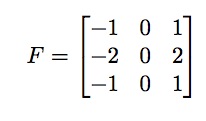
Each number in this filter is referred to as a weight. The weights provided in this filter are example weights. Our goal is to learn the exact weights from the data during convolution. For each convolution layer a set of filters is learned. Use of convolution layer has many features but two stand out:
- Reduction in parameters
In a fully connected neural network the number of parameters is much larger than a convolution network. Consider an image of size 5 x 5 to be convolved with a filter of size, 3 x 3. The number of weights we would have to learn would be the total number of weights in the filter, which is, 9. On the contrary for the same image, using a fully connected layer would require us to learn 225 weights. This is demonstrated in below Figure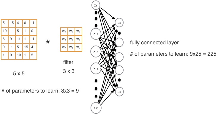
- Exploitation of spatial structure
Our images are in two-dimensions. In order to use them as an input to a fully connected layer, we need to unroll it into a vector and feed it as an input. This leads to the increase in the number of parameters to be learned as shown in the previous section and loss of the original 2D spatial structure. On the contrary, in convolution layer we can directly convolve a 2D image with a 2D filter thereby preserving the original spatial structure and also reducing the number of parameters to be learned.
Implementation Overview
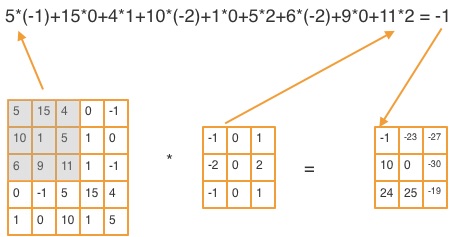
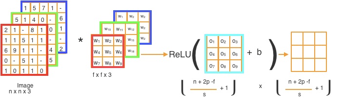
Convolution involves multiplying each pixel in an image by the filter at each position, then summing them up and adding a bias. The figure below shows a single step of convolving an image with a filter. Each convolution will return a 2D matrix output for each input channel.
For example, if the input matrix is of size nxn and the filter is of size fxf, then the convolution output matrix will be of the size (n-f+1)x(n-f+1). The convolution output size remains the same even when there are more than one channels. For example, if there is an RGB image of size (nxnx3) and a filter of size (3x3x3), both with three channels, the convolution output will still be (n-f+1)x(n-f+1). However, if we convolve an image with more than a single filter then we will get a convolved image for each of those filters. For example, an image of size, (nxnx3), convolved with two filters, each of size, (nxnx3), will result in an output of size, (n-f+1)x(n-f+1)x2.
Padding
You probably noticed that with convolution the image gets shrunk in size. This would be a problem in a large network. However, we can retain the size of convolution output by zero-padding the image as shown in the figure below
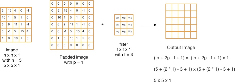
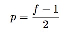
Padding helps to build deeper networks and keep more information at the border of an image. If there is an image of size nxnx1 and it is convolved with a filter of size fxfx1, in order to retain the original size, the output image would have to be of the size (n+2p-f+1) x (n+2p-f+1), where p is the zero-padding size, given by:
Strides
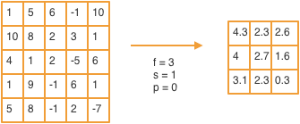
The number of pixels we slide between each step of the convolution of an image and a filter is called a stride. So far we have been sliding one pixel at a time and therefore the stride is 1. However, we could skip a pixel and the stride would be 2, if we skip 2 pixels the stride value will be 3, and so on and so forth. Depending on the value of the stride, the output image has the size,
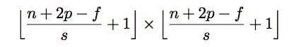
where the input image size is n x n, zero-padded with p columns and rows, with a stride, s, and convolved with a filter of size, f x f.
Pooling layer
The pooling layer shrinks the size of the input image. Reduction in size reduces the computation. Max-pooling layer is demostrated by an example in the below figure
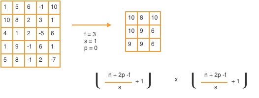
Maxpooling is similar to convolution, except, instead of convolving with a filter, we get the max value in each kernel. In this example, we use a max of f x f kernels of the image, with a padding of 0 and a stride of 1.
Similarly, average pooling takes the average of each kernel as shown in teh figure below:
Activation layer
In order to learn complex and non-linear features we often need a non-linear function. One of the most common non-linear functions is a rectified linear unit (ReLU), as shown in Figure below
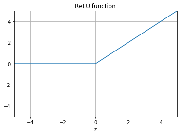
This function is applied to each output of the previous layer and is defined as,
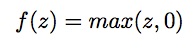
and demonstrated in the following figure
Code
Some of the code is already implemented for you. The details of the starter files that are provided to you are as follows:
- cnnTrain.m
This is the driver file. The data sets are loaded from this file and so are various other functions - cnnCost.m
This file contains the code for backpropagation. It is already implemented for you. - config.m
It is a configuration file where the network components are specified. - All the test code is in the test directory
All of these and other starter code files can be accessed from the following link: https://drive.google.com/drive/folders/1bIbK2fin-6Qnz0Jb_BCxNci1u4kb1umc
What to Implement
You’re supposed to implement the following:
- Forward Pass
Forward pass algorithm to train your Convolution Neural Network. This will work in conjunction with the backpropagation algorithm that is provided to you. You will be implementing this algorithm in cnnConvolve.m file. - Subsampling
After convolution layer, subsample the output by implementing the following two layers in cnnPool.m :- maxpool
- averagepool
- Configuration
Although you wont't need to change either the fully connected layer or the softmax layer you would require more than one convolution and the subsampling layer. In order to add new layers you would have to modify config.m file. The new layers would have to go after the following lines in the file:
cnnConfig.layer{2}.type = 'conv';
cnnConfig.layer{2}.filterDim = [9 9];
cnnConfig.layer{2}.numFilters = 20;
cnnConfig.layer{2}.nonLinearType = 'sigmoid';
cnnConfig.layer{2}.conMatrix = ones(1,20);
cnnConfig.layer{3}.type = 'pool';
cnnConfig.layer{3}.poolDim = [2 2];
cnnConfig.layer{3}.poolType = 'maxpool';
However, make sure you change the index of the subsequent layers since the numbers are sequential.
Submission Guidelines
We will deduct points if your submission does not comply with the following guidelines.
You’re supposed to submit the following:
- All the files that contain your code: cnnConvolve.m, cnnPool.m, config.m or any other files where you implement your code or make modifications.
- Accuracy for a single convolution and subsampling layer with Sigmoid activation function.
- Accuracy for a single convolution and subsampling layer with a ReLu activation function.
- Compare the results between maxpooling and average pooling.
- Try with more than one convolution and subsampling layers for both sigmoid and ReLu activation functions.
- Submit a confusion matrix and the accuracy for the best configuration.
- Dimensions of the Input and output of each layer (convolution(s), maxpool(s) / average pool(s), fully connected layer, and softmax layer) for your best config.
Please submit the project once for your group – there’s no need for each member to submit it.
Collaboration Policy
We encourage you to work closely with your groupmates, including collaborating on writing code. With students outside your group, you may discuss methods and ideas but may not share code.
For the full collaboration policy, including guidelines on citations and limitations on using online resources, see the course website.